Question
The diagram shows the plan of an art gallery a metres wide. [AB] represents a doorway, leading to an exit corridor b metres wide. In order to remove a painting from the art gallery, CD (denoted by L ) is measured for various values of \(\alpha \) , as represented in the diagram.
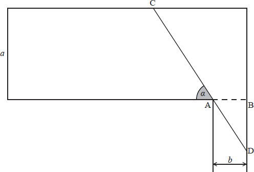
If \(\alpha \) is the angle between [CD] and the wall, show that \(L = \frac{a }{{\sin \alpha }} + \frac{b}{{\cos \alpha }}{\text{, }}0 < \alpha < \frac{\pi }{2}\).
If a = 5 and b = 1, find the maximum length of a painting that can be removed through this doorway.
Let a = 3k and b = k .
Find \(\frac{{{\text{d}}L}}{{{\text{d}}\alpha }}\).
Let a = 3k and b = k .
Find, in terms of k , the maximum length of a painting that can be removed from the gallery through this doorway.
Let a = 3k and b = k .
Find the minimum value of k if a painting 8 metres long is to be removed through this doorway.
Answer/Explanation
Markscheme
\(L = {\text{CA}} + {\text{AD}}\) M1
\({\text{sin}}\alpha {\text{ = }}\frac{a}{{{\text{CA}}}} \Rightarrow {\text{CA}} = \frac{a}{{\sin \alpha }}\) A1
\(\cos \alpha = \frac{b}{{{\text{AD}}}} \Rightarrow {\text{AD}} = \frac{b}{{\cos \alpha }}\) A1
\(L = \frac{a}{{\sin \alpha }} + \frac{b}{{\cos \alpha }}\) AG
[2 marks]
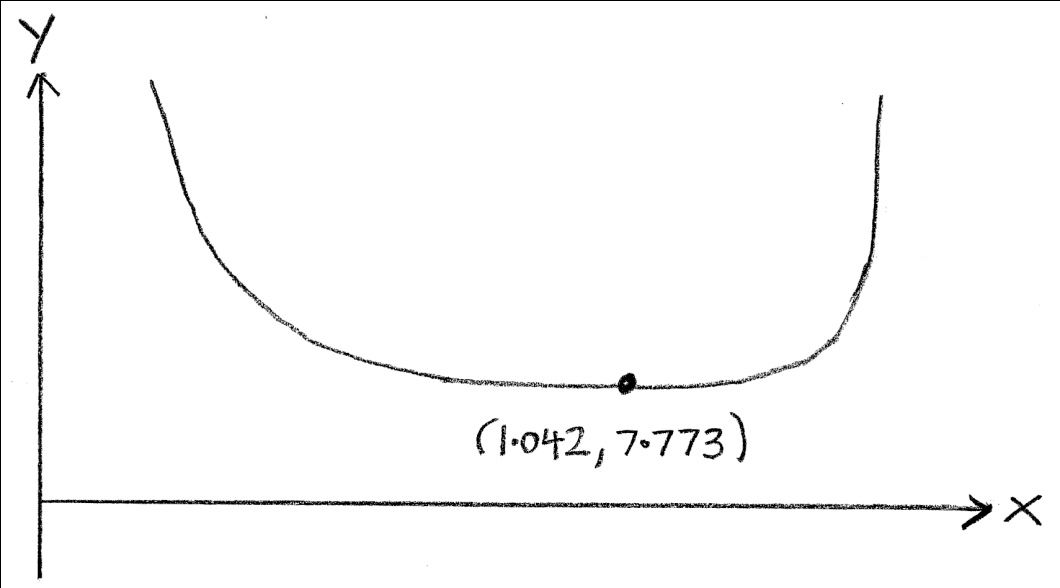
\(a = 5{\text{ and }}b = 1 \Rightarrow L = \frac{5}{{\sin \alpha }} + \frac{1}{{\cos \alpha }}\)
METHOD 1
 (M1)
(M1)
minimum from graph \( \Rightarrow L = 7.77\) (M1)A1
minimum of L gives the max length of the painting R1
[4 marks]
METHOD 2
\(\frac{{{\text{d}}L}}{{{\text{d}}\alpha }} = \frac{{ – 5\cos \alpha }}{{{{\sin }^2}\alpha }} + \frac{{\sin \alpha }}{{{{\cos }^2}\alpha }}\) (M1)
\(\frac{{{\text{d}}L}}{{{\text{d}}\alpha }} = 0 \Rightarrow \frac{{{{\sin }^3}\alpha }}{{{{\cos }^3}\alpha }} = 5 \Rightarrow \tan \alpha = \sqrt[{3{\text{ }}}]{5}{\text{ }}(\alpha = 1.0416…)\) (M1)
minimum of L gives the max length of the painting R1
maximum length = 7.77 A1
[4 marks]
\(\frac{{{\text{d}}L}}{{{\text{d}}\alpha }} = \frac{{ – 3k\cos \alpha }}{{{{\sin }^2}\alpha }} + \frac{{k\sin \alpha }}{{{{\cos }^2}\alpha }}\,\,\,\,\,{\text{(or equivalent)}}\) M1A1A1
[3 marks]
\(\frac{{{\text{d}}L}}{{{\text{d}}\alpha }} = \frac{{ – 3k{{\cos }^3}\alpha + k{{\sin }^3}\alpha }}{{{{\sin }^2}\alpha {{\cos }^2}\alpha }}\) (A1)
\(\frac{{{\text{d}}L}}{{{\text{d}}\alpha }} = 0 \Rightarrow \frac{{{{\sin }^3}\alpha }}{{{{\cos }^3}\alpha }} = \frac{{3k}}{k} \Rightarrow \tan \alpha = \sqrt[3]{3}\,\,\,\,\,(\alpha = 0.96454…)\) M1A1
\(\tan \alpha = \sqrt[3]{3} \Rightarrow \frac{1}{{\cos \alpha }} = \sqrt {1 + \sqrt[3]{9}} \,\,\,\,\,(1.755…)\) (A1)
\({\text{and }}\frac{1}{{\sin \alpha }} = \frac{{\sqrt {1 + \sqrt[3]{9}} }}{{\sqrt[3]{3}}}\,\,\,\,\,(1.216…)\) (A1)
\(L = 3k\left( {\frac{{\sqrt {1 + \sqrt[3]{9}} }}{{\sqrt[3]{3}}}} \right) + k\sqrt {1 + \sqrt[3]{9}} \,\,\,\,\,(L = 5.405598…k)\) A1 N4
[6 marks]
\(L \leqslant 8 \Rightarrow k \geqslant 1.48\) M1A1
the minimum value is 1.48
[2 marks]
Examiners report
Part (a) was very well done by most candidates. Parts (b), (c) and (d) required a subtle balance between abstraction, differentiation skills and use of GDC.
In part (b), although candidates were asked to justify their reasoning, very few candidates offered an explanation for the maximum. Therefore most candidates did not earn the R1 mark in part (b). Also not as many candidates as anticipated used a graphical approach, preferring to use the calculus with varying degrees of success. In part (c), some candidates calculated the derivatives of inverse trigonometric functions. Some candidates had difficulty with parts (d) and (e). In part (d), some candidates erroneously used their alpha value from part (b). In part (d) many candidates used GDC to calculate decimal values for \(\alpha \) and L. The premature rounding of decimals led sometimes to inaccurate results. Nevertheless many candidates got excellent results in this question.
Question
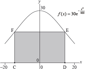
The following diagram shows a vertical cross section of a building. The cross section of the roof of the building can be modelled by the curve \(f(x) = 30{{\text{e}}^{ – \frac{{{x^2}}}{{400}}}}\), where \( – 20 \le x \le 20\).
Ground level is represented by the \(x\)-axis.
Find \(f”(x)\).
Show that the gradient of the roof function is greatest when \(x = – \sqrt {200} \).
The cross section of the living space under the roof can be modelled by a rectangle \(CDEF\) with points \({\text{C}}( – a,{\text{ }}0)\) and \({\text{D}}(a,{\text{ }}0)\), where \(0 < a \le 20\).
Show that the maximum area \(A\) of the rectangle \(CDEF\) is \(600\sqrt 2 {{\text{e}}^{ – \frac{1}{2}}}\).
A function \(I\) is known as the Insulation Factor of \(CDEF\). The function is defined as \(I(a) = \frac{{P(a)}}{{A(a)}}\) where \({\text{P}} = {\text{Perimeter}}\) and \({\text{A}} = {\text{Area of the rectangle}}\).
(i) Find an expression for \(P\) in terms of \(a\).
(ii) Find the value of \(a\) which minimizes \(I\).
(iii) Using the value of \(a\) found in part (ii) calculate the percentage of the cross sectional area under the whole roof that is not included in the cross section of the living space.
Answer/Explanation
Markscheme
\(f'(x) = 30{{\text{e}}^{ – \frac{{{x^2}}}{{400}}}} \bullet – \frac{{2x}}{{400}}\;\;\;\left( { = – \frac{{3x}}{{20}}{{\text{e}}^{ – \frac{{{x^2}}}{{400}}}}} \right)\) M1A1
Note: Award M1 for attempting to use the chain rule.
\(f”(x) = – \frac{3}{{20}}{{\text{e}}^{ – \frac{{{x^2}}}{{400}}}} + \frac{{3{x^2}}}{{4000}}{{\text{e}}^{ – \frac{{{x^2}}}{{400}}}}\;\;\;\left( { = \frac{3}{{20}}{{\text{e}}^{ – \frac{{{x^2}}}{{400}}}}\left( {\frac{{{x^2}}}{{200}} – 1} \right)} \right)\) M1A1
Note: Award M1 for attempting to use the product rule.
[4 marks]
the roof function has maximum gradient when \(f”(x) = 0\) (M1)
Note: Award (M1) for attempting to find \(f”\left( { – \sqrt {200} } \right)\).
EITHER
\( = 0\) A1
OR
\(f”(x) = 0 \Rightarrow x = \pm \sqrt {200} \) A1
THEN
valid argument for maximum such as reference to an appropriate graph or change in the sign of \(f”(x)\) eg \(f”( – 15) = 0.010 \ldots ( > 0)\) and \(f”( – 14) = – 0.001 \ldots ( < 0)\) R1
\( \Rightarrow x = – \sqrt {200} \) AG
[3 marks]
\(A = 2a \bullet 30{{\text{e}}^{ – \frac{{{a^2}}}{{400}}}}\;\;\;\left( { = 60a{{\text{e}}^{ – \frac{{{a^2}}}{{400}}}} = – 400g'(a)} \right)\) (M1)(A1)
EITHER
\(\frac{{{\text{d}}A}}{{{\text{d}}a}} = 60a{{\text{e}}^{ – \frac{{{a^2}}}{{400}}}} \bullet – \frac{a}{{200}} + 60{{\text{e}}^{ – \frac{{{a^2}}}{{400}}}} = 0 \Rightarrow a = \sqrt {200} {\text{ }}\left( { – 400f”(a) = 0 \Rightarrow a = \sqrt {200} } \right)\) M1A1
OR
by symmetry eg \(a = – \sqrt {200} \) found in (b) or \({A_{{\text{max}}}}\) coincides with \(f”(a) = 0\) R1
\( \Rightarrow a = \sqrt {200} \) A1
Note: Award A0(M1)(A1)M0M1 for candidates who start with \(a = \sqrt {200} \) and do not provide any justification for the maximum area. Condone use of \(x\).
THEN
\({A_{{\text{max}}}} = 60 \bullet \sqrt {200} {{\text{e}}^{ – \frac{{200}}{{400}}}}\) M1
\( = 600\sqrt 2 {{\text{e}}^{ – \frac{1}{2}}}\) AG
[5 marks]
(i) perimeter \( = 4a + 60{{\text{e}}^{ – \frac{{{a^2}}}{{400}}}}\) A1A1
Note: Condone use of \(x\).
(ii) \(I(a) = \frac{{4a + 60{{\text{e}}^{ – \frac{{{a^2}}}{{400}}}}}}{{60a{{\text{e}}^{ – \frac{{{a^2}}}{{400}}}}}}\) (A1)
graphing \(I(a)\) or other valid method to find the minimum (M1)
\(a = 12.6\) A1
(iii) area under roof \( = \int_{ – 20}^{20} {30{{\text{e}}^{ – \frac{{{x^2}}}{{400}}}}} {\text{d}}x\) M1
\( = 896.18 \ldots \) (A1)
area of living space \( = 60 \cdot (12.6…) \cdot e – {\frac{{(12.6…)}}{{400}}^2} = 508.56…\)
percentage of empty space \( = 43.3\% \) A1
[9 marks]
Total [21 marks]
Examiners report
[N/A]
[N/A]
[N/A]
[N/A]
Question
A water trough which is 10 metres long has a uniform cross-section in the shape of a semicircle with radius 0.5 metres. It is partly filled with water as shown in the following diagram of the cross-section. The centre of the circle is O and the angle KOL is \(\theta \) radians.
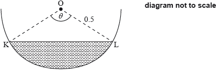
The volume of water is increasing at a constant rate of \(0.0008{\text{ }}{{\text{m}}^3}{{\text{s}}^{ – 1}}\).
Find an expression for the volume of water \(V{\text{ }}({{\text{m}}^3})\) in the trough in terms of \(\theta \).
Calculate \(\frac{{{\text{d}}\theta }}{{{\text{d}}t}}\) when \(\theta = \frac{\pi }{3}\).
Answer/Explanation
Markscheme
area of segment \( = \frac{1}{2} \times {0.5^2} \times (\theta – \sin \theta )\) M1A1
\(V = {\text{area of segment}} \times 10\)
\(V = \frac{5}{4}(\theta – \sin \theta )\) A1
[3 marks]
METHOD 1
\(\frac{{{\text{d}}V}}{{{\text{d}}t}} = \frac{5}{4}(1 – \cos \theta )\frac{{{\text{d}}\theta }}{{{\text{d}}t}}\) M1A1
\(0.0008 = \frac{5}{4}\left( {1 – \cos \frac{\pi }{3}} \right)\frac{{{\text{d}}\theta }}{{{\text{d}}t}}\) (M1)
\(\frac{{{\text{d}}\theta }}{{{\text{d}}t}} = 0.00128{\text{ }}({\text{rad}}\,{s^{ – 1}})\) A1
METHOD 2
\(\frac{{{\text{d}}\theta }}{{{\text{d}}t}} = \frac{{{\text{d}}\theta }}{{{\text{d}}V}} \times \frac{{{\text{d}}V}}{{{\text{d}}t}}\) (M1)
\(\frac{{{\text{d}}V}}{{{\text{d}}\theta }} = \frac{5}{4}(1 – \cos \theta )\) A1
\(\frac{{{\text{d}}\theta }}{{{\text{d}}t}} = \frac{{4 \times 0.0008}}{{5\left( {1 – \cos \frac{\pi }{3}} \right)}}\) (M1)
\(\frac{{{\text{d}}\theta }}{{{\text{d}}t}} = 0.00128\left( {\frac{4}{{3125}}} \right)({\text{rad }}{s^{ – 1}})\) A1
[4 marks]
Examiners report
[N/A]
[N/A]
Question
Consider \(f(x) = – 1 + \ln \left( {\sqrt {{x^2} – 1} } \right)\)
The function \(f\) is defined by \(f(x) = – 1 + \ln \left( {\sqrt {{x^2} – 1} } \right),{\text{ }}x \in D\)
The function \(g\) is defined by \(g(x) = – 1 + \ln \left( {\sqrt {{x^2} – 1} } \right),{\text{ }}x \in \left] {1,{\text{ }}\infty } \right[\).
Find the largest possible domain \(D\) for \(f\) to be a function.
Sketch the graph of \(y = f(x)\) showing clearly the equations of asymptotes and the coordinates of any intercepts with the axes.
Explain why \(f\) is an even function.
Explain why the inverse function \({f^{ – 1}}\) does not exist.
Find the inverse function \({g^{ – 1}}\) and state its domain.
Find \(g'(x)\).
Hence, show that there are no solutions to \(g'(x) = 0\);
Hence, show that there are no solutions to \(({g^{ – 1}})'(x) = 0\).
Answer/Explanation
Markscheme
\({x^2} – 1 > 0\) (M1)
\(x < – 1\) or \(x > 1\) A1
[2 marks]
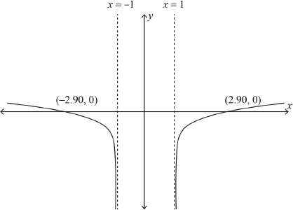
shape A1
\(x = 1\) and \(x = – 1\) A1
\(x\)-intercepts A1
[3 marks]
EITHER
\(f\) is symmetrical about the \(y\)-axis R1
OR
\(f( – x) = f(x)\) R1
[1 mark]
EITHER
\(f\) is not one-to-one function R1
OR
horizontal line cuts twice R1
Note: Accept any equivalent correct statement.
[1 mark]
\(x = – 1 + \ln \left( {\sqrt {{y^2} – 1} } \right)\) M1
\({{\text{e}}^{2x + 2}} = {y^2} – 1\) M1
\({g^{ – 1}}(x) = \sqrt {{{\text{e}}^{2x + 2}} + 1} ,{\text{ }}x \in \mathbb{R}\) A1A1
[4 marks]
\(g'(x) = \frac{1}{{\sqrt {{x^2} – 1} }} \times \frac{{2x}}{{2\sqrt {{x^2} – 1} }}\) M1A1
\(g'(x) = \frac{x}{{{x^2} – 1}}\) A1
[3 marks]
\(g'(x) = \frac{x}{{{x^2} – 1}} = 0 \Rightarrow x = 0\) M1
which is not in the domain of \(g\) (hence no solutions to \(g'(x) = 0\)) R1
[2 marks]
\(({g^{ – 1}})'(x) = \frac{{{{\text{e}}^{2x + 2}}}}{{\sqrt {{{\text{e}}^{2x + 2}} + 1} }}\) M1
as \({{\text{e}}^{2x + 2}} > 0 \Rightarrow ({g^{ – 1}})'(x) > 0\) so no solutions to \(({g^{ – 1}})'(x) = 0\) R1
Note: Accept: equation \({{\text{e}}^{2x + 2}} = 0\) has no solutions.
[2 marks]
Examiners report
[N/A]
[N/A]
[N/A]
[N/A]
[N/A]
[N/A]
[N/A]
[N/A]
Question
Consider \(f(x) = – 1 + \ln \left( {\sqrt {{x^2} – 1} } \right)\)
The function \(f\) is defined by \(f(x) = – 1 + \ln \left( {\sqrt {{x^2} – 1} } \right),{\text{ }}x \in D\)
The function \(g\) is defined by \(g(x) = – 1 + \ln \left( {\sqrt {{x^2} – 1} } \right),{\text{ }}x \in \left] {1,{\text{ }}\infty } \right[\).
Find the largest possible domain \(D\) for \(f\) to be a function.
Sketch the graph of \(y = f(x)\) showing clearly the equations of asymptotes and the coordinates of any intercepts with the axes.
Explain why \(f\) is an even function.
Explain why the inverse function \({f^{ – 1}}\) does not exist.
Find the inverse function \({g^{ – 1}}\) and state its domain.
Find \(g'(x)\).
Hence, show that there are no solutions to \(g'(x) = 0\);
Hence, show that there are no solutions to \(({g^{ – 1}})'(x) = 0\).
Answer/Explanation
Markscheme
\({x^2} – 1 > 0\) (M1)
\(x < – 1\) or \(x > 1\) A1
[2 marks]
shape A1
\(x = 1\) and \(x = – 1\) A1
\(x\)-intercepts A1
[3 marks]
EITHER
\(f\) is symmetrical about the \(y\)-axis R1
OR
\(f( – x) = f(x)\) R1
[1 mark]
EITHER
\(f\) is not one-to-one function R1
OR
horizontal line cuts twice R1
Note: Accept any equivalent correct statement.
[1 mark]
\(x = – 1 + \ln \left( {\sqrt {{y^2} – 1} } \right)\) M1
\({{\text{e}}^{2x + 2}} = {y^2} – 1\) M1
\({g^{ – 1}}(x) = \sqrt {{{\text{e}}^{2x + 2}} + 1} ,{\text{ }}x \in \mathbb{R}\) A1A1
[4 marks]
\(g'(x) = \frac{1}{{\sqrt {{x^2} – 1} }} \times \frac{{2x}}{{2\sqrt {{x^2} – 1} }}\) M1A1
\(g'(x) = \frac{x}{{{x^2} – 1}}\) A1
[3 marks]
\(g'(x) = \frac{x}{{{x^2} – 1}} = 0 \Rightarrow x = 0\) M1
which is not in the domain of \(g\) (hence no solutions to \(g'(x) = 0\)) R1
[2 marks]
\(({g^{ – 1}})'(x) = \frac{{{{\text{e}}^{2x + 2}}}}{{\sqrt {{{\text{e}}^{2x + 2}} + 1} }}\) M1
as \({{\text{e}}^{2x + 2}} > 0 \Rightarrow ({g^{ – 1}})'(x) > 0\) so no solutions to \(({g^{ – 1}})'(x) = 0\) R1
Note: Accept: equation \({{\text{e}}^{2x + 2}} = 0\) has no solutions.
[2 marks]
Examiners report
[N/A]
[N/A]
[N/A]
[N/A]
[N/A]
[N/A]
[N/A]
[N/A]