IB DP Maths Topic 7.1 Geometric distribution HL Paper 3

Question

In a game there are n players, where \(n > 2\) . Each player has a disc, one side of which is red and one side blue. When thrown, the disc is equally likely to show red or blue. All players throw their discs simultaneously. A player wins if his disc shows a different colour from all the other discs. Players throw repeatedly until one player wins.

Let X be the number of throws each player makes, up to and including the one on which the game is won.

(a)     State the distribution of X .

(b)     Find \({\text{P}}(X = x)\) in terms of n and x .

(c)     Find \({\text{E}}(X)\) in terms of n .

(d)     Given that n = 7 , find the least number, k , such that \({\text{P}}(X \leqslant k) > 0.5\) .

▶️Answer/Explanation

Markscheme

(a)     geometric distribution     A1

[1 mark]


(b)     let R be the event throwing the disc and it landing on red and 

let B be the event throwing the disc and it landing on blue 

\({\text{P}}(X = 1) = p = {\text{P}}\left( {1B{\text{ and }}(n – 1)R{\text{ or }}1R{\text{ and }}(n – 1)B} \right)\)     (M1)

\( = n \times \frac{1}{2} \times {\left( {\frac{1}{2}} \right)^{n – 1}} + n \times \frac{1}{2} \times {\left( {\frac{1}{2}} \right)^{n – 1}}\)     (A1)

\( = \frac{n}{{{2^{n – 1}}}}\)     A1

hence \({\text{P}}(X = x) = \frac{n}{{{2^{n – 1}}}}{\left( {1 – \frac{n}{{{2^{n – 1}}}}} \right)^{x – 1}},{\text{ }}(x \geqslant 1)\)     A1

Notes: \(x \geqslant 1\) not required for final A1.

Allow FT for final A1.


[4 marks]


(c)     \({\text{E}}(X) = \frac{1}{p}\)

\( = \frac{{{2^{n – 1}}}}{n}\)     A1

[1 mark]


(d)     when \(n = 7\) , \({\text{P}}(X = x) = {\left( {1 – \frac{7}{{64}}} \right)^{x – 1}} \times \frac{7}{{64}}\)     (M1)

\( = \frac{7}{{64}} \times {\left( {\frac{{57}}{{64}}} \right)^{x – 1}}\)

\({\text{P}}(X \leqslant k) = \sum\limits_{x = 1}^k {\frac{7}{{64}} \times {{\left( {\frac{{57}}{{64}}} \right)}^{x – 1}}} \)     (M1)(A1)

\( \Rightarrow \frac{7}{{64}} \times \frac{{1 – {{\left( {\frac{{57}}{{64}}} \right)}^k}}}{{1 – \frac{{57}}{{64}}}} > 0.5\)     (M1)(A1)

\( \Rightarrow 1 – {\left( {\frac{{57}}{{64}}} \right)^k} > 0.5\)

\( \Rightarrow {\left( {\frac{{57}}{{64}}} \right)^k} < 0.5\)

\( \Rightarrow k > \frac{{\log 0.5}}{{\log \frac{{57}}{{64}}}}\)     (M1)

\( \Rightarrow k > 5.98\)     (A1)

\( \Rightarrow k = 6\)     A1

Note: Tabular and other GDC methods are acceptable.


[8 marks]

Total [14 marks]

Examiners report

This question was found difficult by the majority of candidates and few fully correct answers were seen. Few candidates were able to find \({\text{P}}(X = x)\) in terms of n and x and many did not realise that the last part of the question required them to find the sum of a series. However, better candidates received over 75% of the marks because the answers could be followed through.

Question

The random variable X has a geometric distribution with parameter p .

a.Show that \({\text{P}}(X \leqslant n) = 1 – {(1 – p)^n},{\text{ }}n \in {\mathbb{Z}^ + }\) .[3]


b.Deduce an expression for \({\text{P}}(m < X \leqslant n)\,,{\text{ }}m\,,{\text{ }}n \in {\mathbb{Z}^ + }\) and m < n .[1]


c.Given that p = 0.2, find the least value of n for which \({\text{P}}(1 < X \leqslant n) > 0.5\,,{\text{ }}n \in {\mathbb{Z}^ + }\) .[2]

 
▶️Answer/Explanation

Markscheme

\({\text{P}}(X \leqslant n) = \sum\limits_{{\text{i}} = 1}^n {{\text{P}}(X = {\text{i}}) = \sum\limits_{{\text{i}} = 1}^n {p{q^{{\text{i}} – 1}}} } \)     M1A1

\( = p\frac{{1 – {q^n}}}{{1 – q}}\)     A1

\( = 1 – {(1 – p)^n}\)     AG

[3 marks]

a.

\({(1 – p)^m} – {(1 – p)^n}\)     A1

[1 mark]

b.

attempt to solve \(0.8 – {(0.8)^n} > 0.5\)     M1

obtain n = 6     A1

[2 marks]


Question

Jenny and her Dad frequently play a board game. Before she can start Jenny has to throw a “six” on an ordinary six-sided dice. Let the random variable X denote the number of times Jenny has to throw the dice in total until she obtains her first “six”.

a.If the dice is fair, write down the distribution of X , including the value of any parameter(s).[1]

b.Write down E(X ) for the distribution in part (a).[1]

d.Before Jenny’s Dad can start, he has to throw two “sixes” using a fair, ordinary six-sided dice. Let the random variable Y denote the total number of times Jenny’s Dad has to throw the dice until he obtains his second “six”.

Write down the distribution of Y , including the value of any parameter(s).[1]

e.Before Jenny’s Dad can start, he has to throw two “sixes” using a fair, ordinary six-sided dice. Let the random variable Y denote the total number of times Jenny’s Dad has to throw the dice until he obtains his second “six”.

Find the value of y such that \({\text{P}}(Y = y) = \frac{1}{{36}}\).[1]

f.Before Jenny’s Dad can start, he has to throw two “sixes” using a fair, ordinary six-sided dice. Let the random variable Y denote the total number of times Jenny’s Dad has to throw the dice until he obtains his second “six”.

Find \({\text{P}}(Y \leqslant 6)\) .[2]

 
▶️Answer/Explanation

Markscheme

\(X \sim {\text{Geo}}\left( {\frac{1}{6}} \right){\text{ or NB}}\left( {1,\frac{1}{6}} \right)\)     A1

[1 mark]

a.

\({\text{E}}(X) = 6\)     A1

[1 mark]

b.

Y is \({\text{NB}}\left( {2,\frac{1}{6}} \right)\)     A1

[1 mark]

d.

\({\text{P}}(Y = y) = \frac{1}{{36}}{\text{ gives }}y = 2\)     A1

(as all other probabilities would have a factor of 5 in the numerator)

[1 mark]

e.

\({\text{P}}(Y \leqslant 6) = {\left( {\frac{1}{6}} \right)^2} + 2\left( {\frac{5}{6}} \right){\left( {\frac{1}{6}} \right)^2} + 3{\left( {\frac{5}{6}} \right)^2}{\left( {\frac{1}{6}} \right)^2} + 4{\left( {\frac{5}{6}} \right)^3}{\left( {\frac{1}{6}} \right)^2} + 5{\left( {\frac{5}{6}} \right)^4}{\left( {\frac{1}{6}} \right)^2}\)     (M1)

\( = 0.263\)     A1

[2 marks]


Question

Consider the random variable \(X \sim {\text{Geo}}(p)\).

(a)     State \({\text{P}}(X < 4)\).

(b)     Show that the probability generating function for X is given by \({G_X}(t) = \frac{{pt}}{{1 – qt}}\), where \(q = 1 – p\).

Let the random variable \(Y = 2X\).

(c)     (i)     Show that the probability generating function for Y is given by \({G_Y}(t) = {G_X}({t^2})\).

          (ii)     By considering \({G’_Y}(1)\), show that \({\text{E}}(Y) = 2{\text{E}}(X)\).

Let the random variable \(W = 2X + 1\).

(d)     (i)     Find the probability generating function for W in terms of the probability generating function of Y.

          (ii)     Hence, show that \({\text{E}}(W) = 2{\text{E}}(X) + 1\).

▶️Answer/Explanation

Markscheme

(a)     use of \({\text{P}}(X = n) = p{q^{n – 1}}{\text{ }}(q = 1 – p)\)     (M1)

\({\text{P}}(X < 4) = p + pq + p{q^2}{\text{ }}\left( { = 1 – {q^3}} \right){\text{ }}\left( { = 1 – {{(1 – p)}^3}} \right){\text{ }}( = 3p – 3{p^2} + {p^3})\)     A1

[2 marks]


(b)   \({G_X}(t) = {\text{P}}(X = 1)t + {\text{P}}(X = 2){t^2} +  \ldots \)     (M1)

\( = pt + pq{t^2} + p{q^2}{t^3} +  \ldots \)     A1

summing an infinite geometric series     M1

\( = \frac{{pt}}{{1 – qt}}\)     AG

[3 marks]


(c)     (i)     EITHER

          \({G_Y}(t) = {\text{P}}(Y = 1)t + {\text{P}}(Y = 2){t^2} +  \ldots \)     A1

          \( = 0 \times t + {\text{P}}(X = 1){t^2} + 0 \times {t^3} + {\text{P}}(X = 2){t^4} +  \ldots \)     M1A1

          \( = {G_X}({t^2})\)     AG

          OR

          \({G_Y}(t) = E({t^Y}) = E({t^{2X}})\)     M1A1

          \( = E\left( {{{({t^2})}^X}} \right)\)     A1

          \( = {G_X}({t^2})\)     AG

          (ii)     \({\text{E}}(Y) = {G’_Y}(1)\)     A1

          EITHER

          \( = 2t{G’_X}({t^2})\) evaluated at \(t = 1\)     M1A1

          \( = 2{\text{E}}(X)\)     AG

          OR

          \( = \frac{{\text{d}}}{{{\text{d}}x}}\left( {\frac{{p{t^2}}}{{(1 – q{t^2})}}} \right) = \frac{{2pt(1 – q{t^2}) + 2pq{t^3}}}{{{{(1 – q{t^2})}^2}}}\) evaluated at \(t = 1\)     A1

          \( = 2 \times \frac{{p(1 – qt) + pqt}}{{{{(1 – qt)}^2}}}\) evaluated at \(t = 1{\text{ (or }}\frac{2}{p})\)     A1

          \( = 2{\text{E}}(X)\)     AG

[6 marks]


(d)     (i)     \({G_W}(t) = t{G_Y}(t)\) (or equivalent)     A2

          (ii)     attempt to evaluate \({G’_W}(t)\)     M1

          EITHER

          obtain \(1 \times {G_Y}(t) + t \times {G’_Y}(t)\)     A1

          substitute \(t = 1\) to obtain \(1 \times 1 + 1 \times {G’_Y}(1)\)     A1

          OR

          \( = \frac{{\text{d}}}{{{\text{d}}x}}\left( {\frac{{p{t^3}}}{{(1 – q{t^2})}}} \right) = \frac{{3p{t^2}(1 – q{t^2}) + 2pq{t^4}}}{{{{(1 – q{t^2})}^2}}}\)     A1

          substitute \(t = 1\) to obtain \(1 + \frac{2}{p}\)     A1

          \( = 1 + 2{\text{E}}(X)\)     AG

[5 marks]


Total [16 marks]

Examiners report

[N/A]

Question

A continuous random variable \(T\) has a probability density function defined by

\(f(t) = \left\{ {\begin{array}{*{20}{c}} {\frac{{t(4 – {t^2})}}{4}}&{0 \leqslant t \leqslant 2} \\ {0,}&{{\text{otherwise}}} \end{array}} \right.\).

a.Find the cumulative distribution function \(F(t)\), for \(0 \leqslant t \leqslant 2\).[3]

b.i.Sketch the graph of \(F(t)\) for \(0 \leqslant t \leqslant 2\), clearly indicating the coordinates of the endpoints.[2]

b.ii.Given that \(P(T < a) = 0.75\), find the value of \(a\).[2]

▶️Answer/Explanation

Markscheme

\(F(t) = \int_0^t {\left( {x – \frac{{{x^3}}}{4}} \right){\text{d}}x{\text{ }}\left( { = \int_0^t {\frac{{x(4 – {x^2})}}{4}{\text{d}}x} } \right)} \)     M1

\( = \left[ {\frac{{{x^2}}}{2} – \frac{{{x^4}}}{{16}}} \right]_0^t{\text{ }}\left( { = \left[ {\frac{{{x^2}(8 – {x^2})}}{{16}}} \right]_0^t} \right){\text{ }}\left( { = \left[ {\frac{{ – 4 – {x^2}{)^2}}}{{16}}} \right]_0^t} \right)\)     A1

\( = \frac{{{t^2}}}{2} – \frac{{{t^4}}}{{16}}{\text{ }}\left( { = \frac{{{t^2}(8 – {t^2})}}{{16}}} \right){\text{ }}\left( { = 1 – \frac{{{{(4 – {t^2})}^2}}}{{16}}} \right)\)     A1

Note:     Condone integration involving \(t\) only.

Note:     Award M1A0A0 for integration without limits eg, \(\int {\frac{{t(4 – {t^2})}}{4}{\text{d}}t = \frac{{{t^2}}}{2} – \frac{{{t^4}}}{{16}}} \) or equivalent.

Note:     But allow integration \( + \) \(C\) then showing \(C = 0\) or even integration without \(C\) if \(F(0) = 0\) or \(F(2) = 1\) is confirmed.

[3 marks]

a.

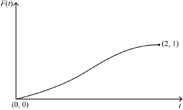
correct shape including correct concavity     A1

clearly indicating starts at origin and ends at \((2,{\text{ }}1)\)     A1

Note:     Condone the absence of \((0,{\text{ }}0)\).

Note:     Accept 2 on the \(x\)-axis and 1 on the \(y\)-axis correctly placed.

[2 marks]

b.i.

attempt to solve \(\frac{{{a^2}}}{2} – \frac{{{a^4}}}{{16}} = 0.75\) (or equivalent) for \(a\)     (M1)

\(a = 1.41{\text{ }}( = \sqrt 2 )\)     A1

Note:     Accept any answer that rounds to 1.4.

[2 marks]

b.ii.

Examiners report

[N/A]

a.

[N/A]

b.i.

[N/A]

b.ii.

Question

Consider an unbiased tetrahedral (four-sided) die with faces labelled 1, 2, 3 and 4 respectively.

The random variable X represents the number of throws required to obtain a 1.

a.State the distribution of X.[1]

b.Show that the probability generating function, \(G\left( t \right)\), for X is given by \(G\left( t \right) = \frac{t}{{4 – 3t}}\).[4]

c.Find \(G’\left( t \right)\).[2]

d.Determine the mean number of throws required to obtain a 1.[1]

▶️Answer/Explanation

Markscheme

X is geometric (or negative binomial)      A1

[1 mark]

a.

\(G\left( t \right) = \frac{1}{4}t + \frac{1}{4}\left( {\frac{3}{4}} \right){t^2} + \frac{1}{4}{\left( {\frac{3}{4}} \right)^2}{t^3} +  \ldots \)     M1A1

recognition of GP \(\left( {{u_1} = \frac{1}{4}t,\,\,r = \frac{3}{4}t} \right)\)     (M1)

\( = \frac{{\frac{1}{4}t}}{{1 – \frac{3}{4}t}}\)     A1

leading to \(G\left( t \right) = \frac{t}{{4 – 3t}}\)     AG

[4 marks]

b.

attempt to use product or quotient rule      M1

\(G’\left( t \right) = \frac{4}{{{{\left( {4 – 3t} \right)}^2}}}\)     A1

[2 marks]

c.

4      A1

Note: Award A1FT to a candidate that correctly calculates the value of \(G’\left( 1 \right)\) from their \(G’\left( t \right)\).

[1 mark]


Scroll to Top