Question
The figure below shows the lengths in centimetres of fish found in the net of a small trawler.
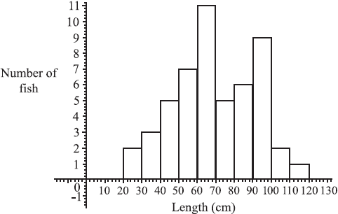
Find the total number of fish in the net.[2]
Find (i) the modal length interval,
(ii) the interval containing the median length,
(iii) an estimate of the mean length.[5]
(i) Write down an estimate for the standard deviation of the lengths.
(ii) How many fish (if any) have length greater than three standard deviations above the mean?[3]
The fishing company must pay a fine if more than 10% of the catch have lengths less than 40cm.
Do a calculation to decide whether the company is fined.[2]
A sample of 15 of the fish was weighed. The weight, W was plotted against length, L as shown below.
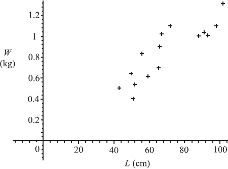
Exactly two of the following statements about the plot could be correct. Identify the two correct statements.
Note: You do not need to enter data in a GDC or to calculate r exactly.
(i) The value of r, the correlation coefficient, is approximately 0.871.
(ii) There is an exact linear relation between W and L.
(iii) The line of regression of W on L has equation W = 0.012L + 0.008 .
(iv) There is negative correlation between the length and weight.
(v) The value of r, the correlation coefficient, is approximately 0.998.
(vi) The line of regression of W on L has equation W = 63.5L + 16.5.[2]
Answer/Explanation
Markscheme
Total = 2 + 3 + 5 + 7 + 11 + 5 + 6 + 9 + 2 + 1 (M1)
(M1) is for a sum of frequencies.
= 51 (A1)(G2)[2 marks]
Unit penalty (UP) is applicable where indicated in the left hand column.
(i) modal interval is 60 – 70
Award (A0) for 65 (A1)
(ii) median is length of fish no. 26, (M1)(A1)
also 60 – 70 (G2)
Can award (A1)(ft) or (G2)(ft) for 65 if (A0) was awarded for 65 in part (i).
(iii) mean is \(\frac{{2 \times 25 + 3 \times 35 + 5 \times 45 + 7 \times 55 + …}}{{51}}\) (M1)
(UP) = 69.5 cm (3sf) (A1)(ft)(G1)
Note: (M1) is for a sum of (frequencies multiplied by midpoint values) divided by candidate’s answer from part (a). Accept mid-points 25.5, 35.5 etc or 24.5, 34.5 etc, leading to answers 70.0 or 69.0 (3sf) respectively. Answers of 69.0, 69.5 or 70.0 (3sf) with no working can be awarded (G1).[5 marks]
Unit penalty (UP) is applicable where indicated in the left hand column.
(UP) (i) standard deviation is 21.8 cm (G1)
For any other answer without working, award (G0). If working is present then (G0)(AP) is possible.
(ii) \(69.5 + 3 \times 21.8 = 134.9 > 120\) (M1)
no fish (A1)(ft)(G1)
For ‘no fish’ without working, award (G1) regardless of answer to (c)(i). Follow through from (c)(i) only if method is shown. [3 marks]
5 fish are less than 40 cm in length, (M1)
Award (M1) for any of \(\frac{5}{51}\), \(\frac{46}{51}\), 0.098 or 9.8%, 0.902, 90.2% or 5.1 seen.
hence no fine. (A1)(ft)
Note: There is no G mark here and (M0)(A1) is never allowed. The follow-through is from answer in part (a).[2 marks]
(i) and (iii) are correct. (A1)(A1)[2 marks]
Question
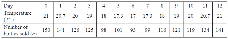
The number of bottles of water sold at a railway station on each day is given in the following table.
Write down
(i) the mean temperature;
(ii) the standard deviation of the temperatures.[2]
Write down the correlation coefficient, \(r\), for the variables \(n\) and \(T\).[1]
Comment on your value for \(r\).[2]
The equation of the line of regression for \(n\) on \(T\) is \(n = dT – 100\).
(i) Write down the value of \(d\).
(ii) Estimate how many bottles of water will be sold when the temperature is \({19.6^ \circ }\).[2]
On a day when the temperature was \({36^ \circ }\) Peter calculates that \(314\) bottles would be sold. Give one reason why his answer might be unreliable.[1]
Answer/Explanation
Markscheme
(i) 19.2 (G1)
(ii) 1.45 (G1)[2 marks]
\(r = 0.942\) (G1)[1 mark]
Strong, positive correlation. (A1)(ft)(A1)(ft)[2 marks]
(i) \(d = 11.5\) (G1)
(ii) \(n = 11.5 \times 19.6 – 100\)
\( = 125\) (accept \(126\)) (A1)(ft)
Note: Answer must be a whole number.[2 marks]
It is unreliable to extrapolate outside the values given (outlier). (R1)[1 mark]
Question
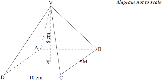
The diagram below shows a square based right pyramid. ABCD is a square of side 10 cm. VX is the perpendicular height of 8 cm. M is the midpoint of BC.
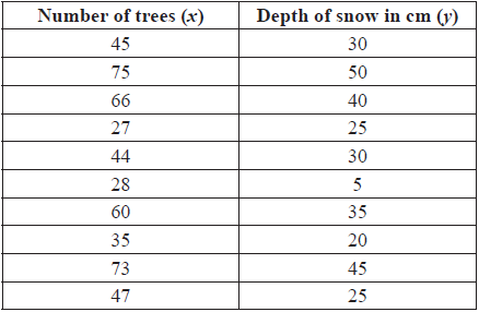
In a mountain region there appears to be a relationship between the number of trees growing in the region and the depth of snow in winter. A set of 10 areas was chosen, and in each area the number of trees was counted and the depth of snow measured. The results are given in the table below.

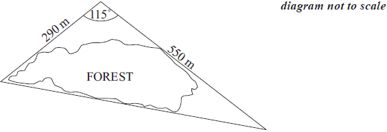
A path goes around a forest so that it forms the three sides of a triangle. The lengths of two sides are 550 m and 290 m. These two sides meet at an angle of 115°. A diagram is shown below.
Write down the length of XM.[1]
Use your graphic display calculator to find the standard deviation of the number of trees.[1]
Calculate the length of VM.[2]
Calculate the angle between VM and ABCD.[2]
Calculate the length of the third side of the triangle. Give your answer correct to the nearest 10 m.[4]
Calculate the area enclosed by the path that goes around the forest.[3]
Inside the forest a second path forms the three sides of another triangle named ABC. Angle BAC is 53°, AC is 180 m and BC is 230 m.
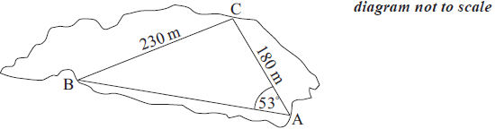
Calculate the size of angle ACB.[4]
Answer/Explanation
Markscheme
UP applies in this question
(UP) XM = 5 cm (A1)[1 mark]
16.8 (G1)[1 mark]
UP applies in this question
VM2 = 52 + 82 (M1)
Note: Award (M1) for correct use of Pythagoras Theorem.
(UP) VM = \(\sqrt{89}\) = 9.43 cm (A1)(ft)(G2)[2 marks]
\(\tan {\text{VMX}} = \frac{8}{5}\) (M1)
Note: Other trigonometric ratios may be used.
\({\rm{V\hat MX}} = 58.0^\circ \) (A1)(ft)(G2)[2 marks]
UP applies in this question
l2 = 2902 + 5502 − 2 × 290 × 550 × cos115° (M1)(A1)
Note: Award (M1) for substituted cosine rule formula, (A1) for correct substitution.
l = 722 (A1)(G2)
(UP) = 720 m (A1)
Note: If 720 m seen without working award (G3).
The final (A1) is awarded for the correct rounding of their answer.[4 marks]
UP applies in this question
\({\text{Area}} = \frac{1}{2} \times 290 \times 550 \times \sin 115\) (M1)(A1)
Note: Award (M1) for substituted correct formula (A1) for correct substitution.
(UP) = \(72\,300{\text{ }}{{\text{m}}^2}\) (A1)(G2)[3 marks]
\(\frac{{180}}{{\sin {\text{B}}}} = \frac{{230}}{{\sin 53}}\) (M1)(A1)
Note: Award (M1) for substituted sine rule formula, (A1) for correct substitution.
B = 38.7° (A1)(G2)
\({\operatorname{A\hat CB}} = 180 – (53^\circ + 38.7^\circ )\)
\( = 88.3^\circ \) (A1)(ft) [4 marks]
Question
In a mountain region there appears to be a relationship between the number of trees growing in the region and the depth of snow in winter. A set of 10 areas was chosen, and in each area the number of trees was counted and the depth of snow measured. The results are given in the table below.
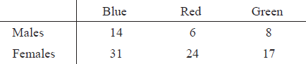
In a study on \(100\) students there seemed to be a difference between males and females in their choice of favourite car colour. The results are given in the table below. A \(\chi^2\) test was conducted.
Use your graphic display calculator to find the mean number of trees.[1]
Use your graphic display calculator to find the mean depth of snow.[1]
Use your graphic display calculator to find the standard deviation of the depth of snow.[1]
The covariance, Sxy = 188.5.
Write down the product-moment correlation coefficient, r.[2]
Write down the equation of the regression line of y on x.[2]
If the number of trees in an area is 55, estimate the depth of snow.[2]
Use the equation of the regression line to estimate the depth of snow in an area with 100 trees.[1]
Decide whether the answer in (e)(i) is a valid estimate of the depth of snow in the area. Give a reason for your answer.[2]
Write down the total number of male students.[1]
Show that the expected frequency for males, whose favourite car colour is blue, is 12.6.[2]
The calculated value of \({\chi ^2}\) is \(1.367\) and the critical value of \({\chi ^2}\) is \(5.99\) at the \(5\%\) significance level.
Write down the null hypothesis for this test.[1]
The calculated value of \({\chi ^2}\) is \(1.367\) and the critical value of \({\chi ^2}\) is \(5.99\) at the \(5\%\) significance level.
Write down the number of degrees of freedom.[1]
The calculated value of \({\chi ^2}\) is \(1.367\) and the critical value of \({\chi ^2}\) is \(5.99\) at the \(5\%\) significance level.
Determine whether the null hypothesis should be accepted at the \(5\%\) significance level. Give a reason for your answer.[2]
Answer/Explanation
Markscheme
50 (G1)[1 mark]
30.5 (G1)[1 mark]
12.3 (G1)
Note: Award (A1)(ft) for 13.0 in (iv) but only if 17.7 seen in (a)(ii).[1 mark]
\(r = \frac{{188.5}}{{(16.79 \times 12.33)}}\) (M1)
Note: Award (M1) for using their values in the correct formula.
= 0.911 (accept 0.912, 0.910) (A1)(ft)(G2)[2 marks]
y = 0.669x − 2.95 (G1)(G1)
Note: Award (G1) for 0.669x, (G1) for −2.95. If the answer is not in the form of an equation, award at most (G1)(G0).[2 marks]
Depth = 0.669 × 55 − 2.95 (M1)
= 33.8 (A1)(ft)(G2)(ft)
Note: Follow through from their (c) even if no working seen.[2 marks]
64.0 (accept 63.95, 63.9) (A1)(ft)(G1)(ft)
Note: Follow through from their (c) even if no working seen.[1 mark]
It is not valid. It lies too far outside the values that are given. Or equivalent. (A1)(R1)
Note: Do not award (A1)(R0).[2 marks]
28 (A1)[1 mark]
\(\frac{{28 \times 45}}{{100}}\left( {\frac{{28}}{{100}} \times \frac{{45}}{{100}} \times 100} \right)\) (M1)(A1)(ft)
Note: Award (M1) for correct formula, (A1) for correct substitution.
= 12.6 (AG)
Note: Do not award (A1) unless 12.6 seen.[2 marks]
the favourite car colour is independent of gender. (A1)
Note: Accept there is no association between gender and favourite car colour.
Do not accept ‘not related’ or ‘not correlated’.[1 mark]
\(2\) (A1)[1 marks]
Accept the null hypothesis since \(1.367 < 5.991\) (A1)(ft)(R1)
Note: Allow “Do not reject”. Follow through from their null hypothesis and their critical value.
Full credit for use of \(p\)-values from GDC [\(p = 0.505\)].
Do not award (A1)(R0). Award (R1) for valid comparison.[2 marks]
Question
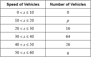
The speed, \(s\) , in \({\text{km }}{{\text{h}}^{ – 1}}\), of \(120\) vehicles passing a point on the road was measured. The results are given below.
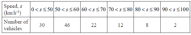
Write down the midpoint of the \(60 < s \leqslant 70\) interval.[1]
Use your graphic display calculator to find an estimate for
(i) the mean speed of the vehicles;
(ii) the standard deviation of the speeds of the vehicles.[3]
Write down the number of vehicles whose speed is less than or equal to \({\text{60 km }}{{\text{h}}^{ – 1}}\).[1]
Consider the cumulative frequency table below.
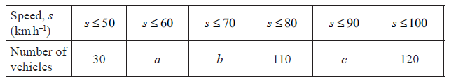
Write down the value of \(a\) , of \(b\) and of \(c\) .[2]
Consider the cumulative frequency table below.

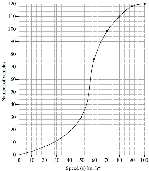
Draw a cumulative frequency graph for the information from the table. Use \(1\) cm to represent \({\text{10 km }}{{\text{h}}^{ – 1}}\) on the horizontal axis and \(1\) cm to represent \(10\) vehicles on the vertical axis.[4]
Use your cumulative frequency graph to estimate
(i) the median speed of the vehicles;
(ii) the number of vehicles that are travelling at a speed less than or equal to \({\text{65 km }}{{\text{h}}^{ – 1}}\).[4]
All drivers whose vehicle’s speed is greater than one standard deviation above the speed limit of \({\text{50 km }}{{\text{h}}^{ – 1}}\) will be fined.
Use your graph to estimate the number of drivers who will be fined.[3]
Answer/Explanation
Markscheme
\(65\) (A1)[1 mark]
(i) \(54{\text{ (km }}{{\text{h}}^{ – 1}})\) (G2)
Note: If the answer to part (b)(i) is consistent with the answer to part (a) then award (G2)(ft) even if no working seen.
(ii) \(19.2\) (\(19.2093 \ldots \)) (G1)
Note: Accept \(19\), do not accept \(20\).[3 marks]
\(76\) (A1)[1 mark]
\(a = 76\), \(b = 98\) (A1)(ft)
Note: Follow through from their answer to part (c) for \(a\) and \(b = \) their \(a + 22\) .
\(c = 118\) (A1)[2 marks]
 (A1)(A1)(ft)(A1)(ft)(A1)
Notes: Award (A1) for axes labelled and correct scales. If the axes are reversed do not award this mark but follow through. Award (A2)(ft) for their 6 points correct, (A1)(ft) for at least 3 of these points correct. Award (A1) for smooth curve drawn through all points including (\(0\), \(0\)). If either the \(x\) or the \(y\) axis has a break in it to zero, do not award this final mark.[4 marks]
(i) \(57\) \({\text{(km }}{{\text{h}}^{ – 1}})\) \(( \pm 2)\) (M1)(A1)(ft)(G2)
Note: Award (M1) for clear indication of median on their graph. Follow through from their graph. If their answer is consistent with their incorrect graph but there is no working present on graph then no marks are awarded.
(ii) \(90\) vehicles \(( \pm 2)\) (M1)(A1)(ft)(G2)
Note: Award (M1) for clear indication of method on their graph. Follow through from their graph. If their answer is consistent with their incorrect graph but there is no working present on graph then no marks are awarded.[4 marks]
\(50 + 19.2 = 69.2\) (A1)(ft)
\(24\) \(( \pm 2)\) drivers will be fined (M1)(A1)(ft)(G2)
Notes: Follow through from their graph and from their part (b)(ii). Award (M1) for indication of method on their graph. If their answer is consistent with their incorrect graph but there is no working present on graph then no marks are awarded.[3 marks]
Question
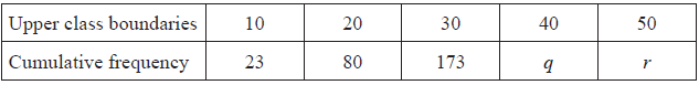
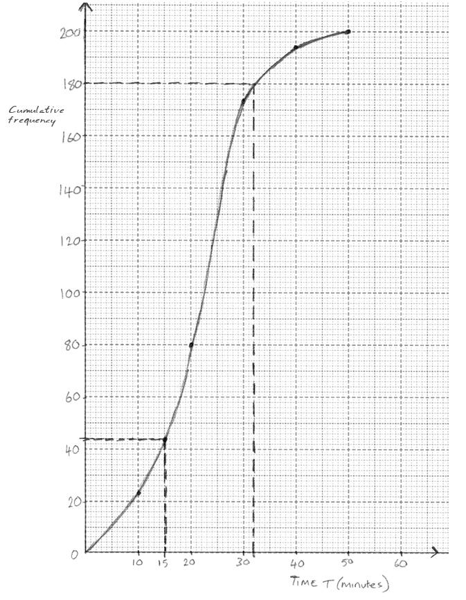
200 people were asked the amount of time T (minutes) they had spent in the supermarket. The results are represented in the table below.
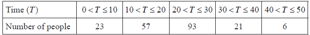
State if the data is discrete or continuous.[1]
State the modal group.[1]
Write down the midpoint of the interval 10 < T ≤ 20 .[1]
Use your graphic display calculator to find an estimate for
(i) the mean;
(ii) the standard deviation.[3]
The results are represented in the cumulative frequency table below, with upper class boundaries of 10, 20, 30, 40, 50.

Write down the value of
(i) q;
(ii) r.[2]
The results are represented in the cumulative frequency table below, with upper class boundaries of 10, 20, 30, 40, 50.
On graph paper, draw a cumulative frequency graph, using a scale of 2 cm to represent 10 minutes (T) on the horizontal axis and 1 cm to represent 10 people on the vertical axis.[4]
Use your graph from part (f) to estimate
(i) the median;
(ii) the 90th percentile of the results;
(iii) the number of people who shopped at the supermarket for more than 15 minutes.[6]
Answer/Explanation
Markscheme
continuous (A1)[1 mark]
20 < T ≤ 30 (A1)[1 mark]
15 (A1)[1 mark]
(i) 21.5 (G2)
(ii) 9.21 (9.20597…) (G1) [3 marks]
(i) q = 194 (A1)
(ii) r = 200 (A1)[2 marks]
 (A1)(A2)(ft)(A1)
Notes: Award (A1) for scale and axis labels, (A2)(ft) for 5 correct points, (A1)(ft) for 4 or 3 correct points, (A0) for less than 3 correct points, (A1) for smooth curve through their points, starting at (0, 0). Follow through from their answers to parts (e)(i) and (e)(ii).[4 marks]
(i) 22.5 ± 2 (A1)
(ii) 32 ± 2 (M1)(A1)(ft)(G2)
Note: Award (M1) for lines drawn on graph or some indication of method, follow through from their graph if working is shown.
(iii) 44 ± 2 (A1)(ft)
Note: Follow through from their graph if working is shown.
200 − 44 = 156 (M1)(A1)(ft)(G2)
Note: Award (M1) for subtraction from 200, follow through from their graph if working is shown.[6 marks]
Question
The table below shows the scores for 12 golfers for their first two rounds in a local golf tournament.
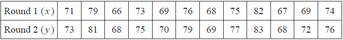
(i) Write down the mean score in Round 1.
(ii) Write down the standard deviation in Round 1.
(iii) Find the number of these golfers that had a score of more than one standard deviation above the mean in Round 1.[5]
Write down the correlation coefficient, r.[2]
Write down the equation of the regression line of y on x.[2]
Another golfer scored 70 in Round 1.
Calculate an estimate of his score in Round 2.[2]
Another golfer scored 89 in Round 1.
Determine whether you can use the equation of the regression line to estimate his score in Round 2. Give a reason for your answer.[2]
Answer/Explanation
Markscheme
(i) \(\frac{{71 + 79 + …}}{{12}}\) (M1)
\(72.4\left( {72.4166…,{\text{ }}\frac{{869}}{{12}}} \right)\) (A1)(G2)
Note: Award (M1) for correct substitution into the mean formula.
(ii) 4.77 (4.76896…) (G1)
(iii) 72.4 + 4.77 = 77.17 (M1)
Note: Award (M1) for adding their mean to their standard deviation.
Two golfers (A1)(ft)(G2)
Note: Follow through from their answers to parts (i) and (ii).[5 marks]
0.990 (0.99014…) (G2)[2 marks]
y = 1.01x + 0.816 (y = 1.01404…x + 0.81618…) (G1)(G1)
Notes: Award (G1) for 1.01x and (G1) for 0.816. If the answer is not an equation award a maximum of (G1)(G0).
OR
y − 74.25 = 1.01(x − 72.4)(y − 74.25 = 1.01404…(x − 72.4166…)) (A1)(A1)
Notes: Award (A1) for 1.01 correctly substituted in the equation, and (A1)(ft) for correct substitution of (72.4, 74.25) in the equation. Follow through from their part (a)(i). If the final answer is not an equation award a maximum of (A1)(A0).[2 marks]
y = 1.01404… × 70 + 0.81618… (M1)
Note: Award (M1) for substitution of 70 into their regression line equation from part (c).
y = 72 (71.7989…) (A1)(ft)(G2)
Note: Follow through from their part (c).[2 marks]
No, equation cannot be (reliably) used as 89 is outside the data range. (A1)(R1)
OR
Yes, but the result is not valid/not reliable as 89 is outside the data range/as we extrapolate (A1)(R1)
Note: Do not award (A1)(R0).[2 marks]
Question
The cumulative frequency graph shows the speed, \(s\), in \({\text{km}}\,{{\text{h}}^{ – 1}}\), of \(120\) vehicles passing a hospital gate.
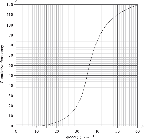
Estimate the minimum possible speed of one of these vehicles passing the hospital gate.[1]
Find the median speed of the vehicles.[2]
Write down the \({75^{{\text{th}}}}\) percentile.[1]
Calculate the interquartile range.[2]
The speed limit past the hospital gate is \(50{\text{ km}}\,{{\text{h}}^{ – 1}}\).
Find the number of these vehicles that exceed the speed limit.[2]
The table shows the speeds of these vehicles travelling past the hospital gate.
Find the value of \(p\) and of \(q\).[2]
The table shows the speeds of these vehicles travelling past the hospital gate.
(i) Write down the modal class.
(ii) Write down the mid-interval value for this class.[2]
The table shows the speeds of these vehicles travelling past the hospital gate.
Use your graphic display calculator to calculate an estimate of
(i) the mean speed of these vehicles;
(ii) the standard deviation.[3]
It is proposed that the speed limit past the hospital gate is reduced to \(40{\text{ km}}\,{{\text{h}}^{ – 1}}\) from the current \(50{\text{ km}}\,{{\text{h}}^{ – 1}}\).
Find the percentage of these vehicles passing the hospital gate that do not exceed the current speed limit but would exceed the new speed limit.[2]
Answer/Explanation
Markscheme
\(10{\text{ (km}}\,{{\text{h}}^{ – 1}})\) (A1)
\(36\) (G2)
\(41.5\) (G1)
\(41.5 – 32.5\) (M1)
\( = 9{\text{ (}} \pm {\text{1)}}\) (A1)(ft)(G2)
Notes: Award (M1) for quartiles seen. Follow through from part (c).
\(120 – 110\) (M1)
\( = 10\) (A1)(G2)
Note: Award (M1) for \(110\) seen.
\(p = 4\;\;\;q = 10\) (A1)(ft)(A1)(ft)
Note: Follow through from part (e).
(i) \(30 < s \leqslant 40\) (A1)
(ii) \(35\) (A1)(ft)
Note: Follow through from part (g)(i).
(i) \(36.8{\text{ (km}}\,{{\text{h}}^{ – 1}})\;\;\;(36.8333)\) (G2)(ft)
Notes: Follow through from part (f).
(ii) \(8.85\;\;\;(8.84904 \ldots )\) (G1)(ft)
Note: Follow through from part (f), irrespective of working seen.
\(\frac{{26}}{{120}} \times 100\) (M1)
Note: Award (M1) for \(\frac{{26}}{{120}} \times 100\) seen.
\( = 21.7{\text{ (}}\% )\;\;\;\left( {21.6666 \ldots ,{\text{ }}21\frac{2}{3},{\text{ }}\frac{{65}}{3}} \right)\) (A1)(G2)
Question
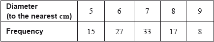
Daniel grows apples and chooses at random a sample of 100 apples from his harvest.
He measures the diameters of the apples to the nearest cm. The following table shows the distribution of the diameters.
Using your graphic display calculator, write down the value of
(i) the mean of the diameters in this sample;
(ii) the standard deviation of the diameters in this sample.[3]
Daniel assumes that the diameters of all of the apples from his harvest are normally distributed with a mean of 7 cm and a standard deviation of 1.2 cm. He classifies the apples according to their diameters as shown in the following table.

Calculate the percentage of small apples in Daniel’s harvest.[3]
Daniel assumes that the diameters of all of the apples from his harvest are normally distributed with a mean of 7 cm and a standard deviation of 1.2 cm. He classifies the apples according to their diameters as shown in the following table.
Of the apples harvested, 5% are large apples.
Find the value of \(a\).[2]
Daniel assumes that the diameters of all of the apples from his harvest are normally distributed with a mean of 7 cm and a standard deviation of 1.2 cm. He classifies the apples according to their diameters as shown in the following table.
Find the percentage of medium apples.[2]
Daniel assumes that the diameters of all of the apples from his harvest are normally distributed with a mean of 7 cm and a standard deviation of 1.2 cm. He classifies the apples according to their diameters as shown in the following table.
This year, Daniel estimates that he will grow \({\text{100}}\,{\text{000}}\) apples.
Estimate the number of large apples that Daniel will grow this year.[2]
Answer/Explanation
Markscheme
(i) \(6.76{\text{ (cm)}}\) (G2)
Notes: Award (M1) for an attempt to use the formula for the mean with a least two rows from the table.
(ii) \(1.14{\text{ (cm)}}\;\;\;\left( {1.14122 \ldots {\text{ (cm)}}} \right)\) (G1)
\({\text{P}}({\text{diameter}} < 6.5) = 0.338\;\;\;(0.338461)\) (M1)(A1)
Notes: Award (M1) for attempting to use the normal distribution to find the probability or for correct region indicated on labelled diagram. Award (A1) for correct probability.
\(33.8(\% )\) (A1)(ft)(G3)
Notes: Award (A1)(ft) for converting their probability into a percentage.
\({\text{P}}({\text{diameter}} \geqslant a) = 0.05\) (M1)
Note: Award (M1) for attempting to use the normal distribution to find the probability or for correct region indicated on labelled diagram.
\(a = 8.97{\text{ (cm)}}\;\;\;(8.97382 \ldots )\) (A1)(G2)
\(100 – (5 + 33.8461 \ldots )\) (M1)
Note: Award (M1) for subtracting “\(5+\) their part (b)” from 100 or (M1) for attempting to use the normal distribution to find the probability \({\text{P}}\left( {6.5 \leqslant {\text{diameter}} < {\text{their part (c)}}} \right)\) or for correct region indicated on labelled diagram.
\( = 61.2(\% )\;\;\;\left( {61.1538 \ldots (\% )} \right)\) (A1)(ft)(G2)
Notes: Follow through from their answer to part (b). Percentage symbol is not required. Accept \(61.1(\%)\) (\(61.1209\ldots(\%)\)) if \(8.97\) used.
\(100\,000 \times 0.05\) (M1)
Note: Award (M1) for multiplying by \(0.05\) (or \(5\%\)).
\( = 5000\) (A1)(G2)
Question
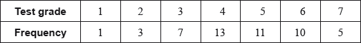
The table below shows the distribution of test grades for 50 IB students at Greendale School.
A student is chosen at random from these 50 students.
A second student is chosen at random from these 50 students.
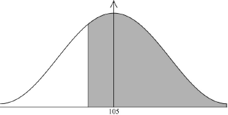
The number of minutes that the 50 students spent preparing for the test was normally distributed with a mean of 105 minutes and a standard deviation of 20 minutes.
Calculate the mean test grade of the students;[2]
Calculate the standard deviation.[1]
Find the median test grade of the students.[1]
Find the interquartile range.[2]
Find the probability that this student scored a grade 5 or higher.[2]
Given that the first student chosen at random scored a grade 5 or higher, find the probability that both students scored a grade 6.[3]
Calculate the probability that a student chosen at random spent at least 90 minutes preparing for the test.[2]
Calculate the expected number of students that spent at least 90 minutes preparing for the test.[2]
Answer/Explanation
Markscheme
\(\frac{{1(1) + 3(2) + 7(3) + 13(4) + 11(5) + 10(6) + 5(7)}}{{50}} = \frac{{230}}{{50}}\) (M1)
Note: Award (M1) for correct substitution into mean formula.
\( = 4.6\) (A1) (G2)[2 marks]
\(1.46{\text{ }}(1.45602 \ldots )\) (G1)[1 mark]
5 (A1)[1 mark]
\(6 – 4\) (M1)
Note: Award (M1) for 6 and 4 seen.
\( = 2\) (A1) (G2)[2 marks]
\(\frac{{11 + 10 + 5}}{{50}}\) (M1)
Note: Award (M1) for \(11 + 10 + 5\) seen.
\( = \frac{{26}}{{50}}{\text{ }}\left( {\frac{{13}}{{25}},{\text{ }}0.52,{\text{ }}52\% } \right)\) (A1) (G2)[2 marks]
\(\frac{{10}}{{{\text{their }}26}} \times \frac{9}{{49}}\) (M1)(M1)
Note: Award (M1) for \(\frac{{10}}{{{\text{their }}26}}\) seen, (M1) for multiplying their first probability by \(\frac{9}{{49}}\).
OR
\(\frac{{\frac{{10}}{{50}} \times \frac{9}{{49}}}}{{\frac{{26}}{{50}}}}\)
Note: Award (M1) for \({\frac{{10}}{{50}} \times \frac{9}{{49}}}\) seen, (M1) for dividing their first probability by \(\frac{{{\text{their }}26}}{{50}}\).
\( = \frac{{45}}{{637}}{\text{ (}}0.0706,{\text{ }}0.0706436 \ldots ,{\text{ }}7.06436 \ldots \% )\) (A1)(ft) (G3)
Note: Follow through from part (d).[3 marks]
\({\text{P}}(X \geqslant 90)\) (M1)
OR
 (M1)
(M1)
Note: Award (M1) for a diagram showing the correct shaded region \(( > 0.5)\).
\(0.773{\text{ }}(0.773372 \ldots ){\text{ }}0.773{\text{ }}(0.773372 \ldots ,{\text{ }}77.3372 \ldots \% )\) (A1) (G2)[2 marks]
\(0.773372 \ldots \times 50\) (M1)
\( = 38.7{\text{ }}(38.6686 \ldots )\) (A1)(ft) (G2)
Note: Follow through from part (f)(i).[2 marks]
Question
A group of 800 students answered 40 questions on a category of their choice out of History, Science and Literature.
For each student the category and the number of correct answers, \(N\), was recorded. The results obtained are represented in the following table.
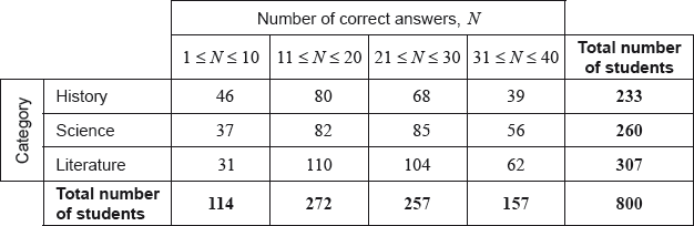
A \({\chi ^2}\) test at the 5% significance level is carried out on the results. The critical value for this test is 12.592.
State whether \(N\) is a discrete or a continuous variable.[1]
Write down, for \(N\), the modal class;[1]
Write down, for \(N\), the mid-interval value of the modal class.[1]
Use your graphic display calculator to estimate the mean of \(N\);[2]
Use your graphic display calculator to estimate the standard deviation of \(N\).[1]
Find the expected frequency of students choosing the Science category and obtaining 31 to 40 correct answers.[2]
Write down the null hypothesis for this test;[1]
Write down the number of degrees of freedom.[1]
Write down the \(p\)-value for the test;[1]
Write down the \({\chi ^2}\) statistic.[2]
State the result of the test. Give a reason for your answer.[2]
Answer/Explanation
Markscheme
discrete (A1)[1 mark]
\(11 \leqslant N \leqslant 20\) (A1)[1 mark]
15.5 (A1)(ft)
Note: Follow through from part (b)(i).[1 mark]
\(21.2{\text{ }}(21.2125)\) (G2)[2 marks]
\(9.60{\text{ }}(9.60428 \ldots )\) (G1)[1 marks]
\(\frac{{260}}{{800}} \times \frac{{157}}{{800}} \times 800\)\(\,\,\,\)OR\(\,\,\,\)\(\frac{{260 \times 157}}{{800}}\) (M1)
Note: Award (M1) for correct substitution into expected frequency formula.
\( = 51.0{\text{ }}(51.025)\) (A1)(G2)[2 marks]
choice of category and number of correct answers are independent (A1)
Notes: Accept “no association” between (choice of) category and number of correct answers. Do not accept “not related” or “not correlated” or “influenced”.[1 mark]
6 (A1)[1 mark]
\(0.0644{\text{ }}(0.0644123 \ldots )\) (G1)[1 mark]
\(11.9{\text{ }}(11.8924 \ldots )\) (G2)[2 marks]
the null hypothesis is not rejected (the null hypothesis is accepted) (A1)(ft)
OR
(choice of) category and number of correct answers are independent (A1)(ft)
as \(11.9 < 12.592\)\(\,\,\,\)OR\(\,\,\,\)\(0.0644 > 0.05\) (R1)
Notes: Award (R1) for a correct comparison of either their \({\chi ^2}\) statistic to the \({\chi ^2}\) critical value or their \(p\)-value to the significance level. Award (A1)(ft) from that comparison.
Follow through from part (f). Do not award (A1)(ft)(R0).[2 marks]
Question
On one day 180 flights arrived at a particular airport. The distance travelled and the arrival status for each incoming flight was recorded. The flight was then classified as on time, slightly delayed, or heavily delayed.
The results are shown in the following table.
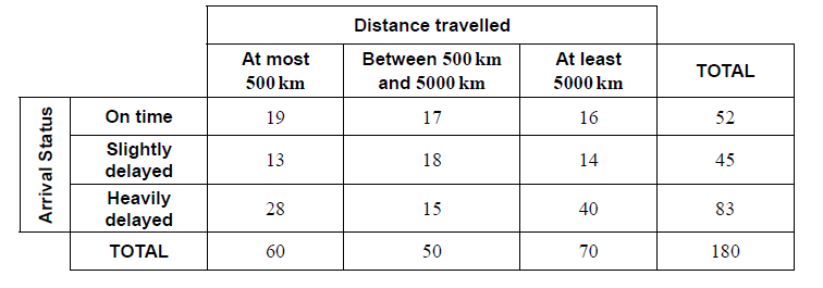
A χ2 test is carried out at the 10 % significance level to determine whether the arrival status of incoming flights is independent of the distance travelled.
The critical value for this test is 7.779.
A flight is chosen at random from the 180 recorded flights.
State the alternative hypothesis.[1]
Calculate the expected frequency of flights travelling at most 500 km and arriving slightly delayed.[2]
Write down the number of degrees of freedom.[1]
Write down the χ2 statistic.[2]
Write down the associated p-value.[1]
State, with a reason, whether you would reject the null hypothesis.[2]
Write down the probability that this flight arrived on time.[2]
Given that this flight was not heavily delayed, find the probability that it travelled between 500 km and 5000 km.[2]
Two flights are chosen at random from those which were slightly delayed.
Find the probability that each of these flights travelled at least 5000 km.[3]
Answer/Explanation
Markscheme
The arrival status is dependent on the distance travelled by the incoming flight (A1)
Note: Accept “associated” or “not independent”.[1 mark]
\(\frac{{60 \times 45}}{{180}}\) OR \(\frac{{60}}{{180}} \times \frac{{45}}{{180}} \times 180\) (M1)
Note: Award (M1) for correct substitution into expected value formula.
= 15 (A1) (G2)[2 marks]
4 (A1)
Note: Award (A0) if “2 + 2 = 4” is seen.[1 mark]
9.55 (9.54671…) (G2)
Note: Award (G1) for an answer of 9.54.[2 marks]
0.0488 (0.0487961…) (G1)[1 mark]
Reject the Null Hypothesis (A1)(ft)
Note: Follow through from their hypothesis in part (a).
9.55 (9.54671…) > 7.779 (R1)(ft)
OR
0.0488 (0.0487961…) < 0.1 (R1)(ft)
Note: Do not award (A1)(ft)(R0)(ft). Follow through from part (d). Award (R1)(ft) for a correct comparison, (A1)(ft) for a consistent conclusion with the answers to parts (a) and (d). Award (R1)(ft) for χ2calc > χ2crit , provided the calculated value is explicitly seen in part (d)(i).[2 marks]
\(\frac{{52}}{{180}}\,\,\left( {0.289,\,\,\frac{{13}}{{45}},\,\,28.9\,{\text{% }}} \right)\) (A1)(A1) (G2)
Note: Award (A1) for correct numerator, (A1) for correct denominator.[2 marks]
\(\frac{{35}}{{97}}\,\,\left( {0.361,\,\,36.1\,{\text{% }}} \right)\) (A1)(A1) (G2)
Note: Award (A1) for correct numerator, (A1) for correct denominator.[2 marks]
\(\frac{{14}}{{45}} \times \frac{{13}}{{44}}\) (A1)(M1)
Note: Award (A1) for two correct fractions and (M1) for multiplying their two fractions.
\( = \frac{{182}}{{1980}}\,\,\left( {0.0919,\,\,\frac{{91}}{{990}},\,0.091919 \ldots ,\,9.19\,{\text{% }}} \right)\) (A1) (G2)[3 marks]
Question
The lengths (\(l\)) in centimetres of \(100\) copper pipes at a local building supplier were measured. The results are listed in the table below.
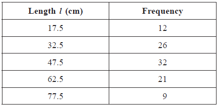
Write down the mode.[1]
Using your graphic display calculator, write down the value of
(i) the mean;
(ii) the standard deviation;
(iii) the median.[4]
Find the interquartile range.[2]
Draw a box and whisker diagram for this data, on graph paper, using a scale of \(1{\text{ cm}}\) to represent \(5{\text{ cm}}\).[4]
Sam estimated the value of the mean of the measured lengths to be \(43{\text{ cm}}\).
Find the percentage error of Sam’s estimated mean.[2]
Answer/Explanation
Markscheme
\(47.5{\text{ (cm)}}\) (A1)
(i) \(45.85{\text{ (cm)}}\) (G2)
Note: Accept \(45.9\) .
(ii) \(17.1{\text{ }}(17.0888 \ldots )\) (G1)
(iii) \(47.5{\text{ (cm)}}\) (G1)
\(62.5 – 32.5 = 30\) (M1)(A1)(G2)Note: Award (M1) for correct quartiles seen.
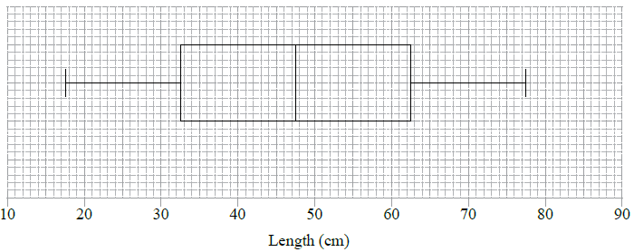
(A1) for correct label and scale
(A1)(ft) for correct median
(A1)(ft) for correct quartiles and box
(A1) for endpoints at \(17.5\) and \(77.5\) joined to box by straight lines (A1)(A1)(ft)(A1)(ft)(A1)
Notes: The final (A1) is lost if the lines go through the box. Follow through from their parts (b) and (c).
\(\varepsilon = \left| {\frac{{43 – 45.85}}{{45.85}}} \right| \times 100\% \) (M1)
Note: Award (M1) for their correct substitution in \(\% \) error formula.
\( = 6.22\% \) (\(6.21592 \ldots \)) (A1)(ft)(G2)
Notes: Follow through from their answer to part (b)(i). Accept \(6.32\% \) with use of \(45.9\) .