New IBDP Mathematics: analysis and approaches courses- Syllabus
Topic 1: Number and algebra– SL content
- Topic : SL 1.1
- Topic : SL 1.2
- Topic : SL 1.3
- Topic : SL 1.4
- Financial applications of geometric sequences and series:
- compound interest
- annual depreciation
- Financial applications of geometric sequences and series:
- Topic : SL 1.5
- Laws of exponents with integer exponents.
- Introduction to logarithms with base 10 and e. Numerical evaluation of logarithms using technology.
- Topic : SL 1.6
- Simple deductive proof, numerical and algebraic; how to lay out a left-hand side to right-hand side (LHS to RHS) proof. The symbols and notation for equality and identity.
- Topic : SL 1.7
- Laws of exponents with rational exponents.
- Laws of logarithms.
- logaxy = logax + logay
- loga\(\frac{x}{y}\)=logax – logay
- logaxm = mlogax for a, x, y > 0
- Change of base of a logarithm.
- logax = \(\frac{log_bx}{log_ba}\) for a, b, x > 0
- Solving exponential equations, including using logarithms
- Topic : SL 1.8
- Sum of infinite convergent geometric sequences.
- Topic : SL 1.9
- The binomial theorem: expansion of (a + b)n , n ∈ ℕ.
- Use of Pascal’s triangle and nCr
Topic 2: Functions– SL content
- Topic: SL 2.1
- Different forms of the equation of a straight line.
- Gradient; intercepts.
- Lines with gradients m1 and m2
- Parallel lines m1 = m2.
- Perpendicular lines m1 × m2 = − 1.
- Topic: SL 2.2
- Concept of a function, domain, range and graph. Function notation, for example f(x), v(t), C(n). The concept of a function as a mathematical model.
- Informal concept that an inverse function reverses or undoes the effect of a function. Inverse function as a reflection in the line y = x, and the notation f−1(x).
- Topic: SL 2.3
- The graph of a function; its equation \(y = f\left( x \right)\) .
- Creating a sketch from information given or a context, including transferring a graph from screen to paper. Using technology to graph functions including their sums and differences.
- Topic: SL 2.4
- Determine key features of graphs.
- Finding the point of intersection of two curves or lines using technology
- Topic: SL 2.5
- Composite functions.
- (f ∘ g)(x) = f(g(x))
- Identity function.
- Finding the inverse function f−1(x)
- (f ∘ f−1)(x) = (f−1∘ f)(x) = x
- Composite functions.
- Topic: SL 2.6
- The quadratic function f(x) = ax2 + bx + c: its graph, y -intercept (0, c). Axis of symmetry.
- The form f(x) = a(x − p)(x − q), x intercepts (p, 0) and (q, 0).The form f(x) = a (x − h) 2 + k, vertex (h,k).
- Topic: SL 2.7
- Solution of quadratic equations and inequalities. The quadratic formula.
- The discriminant \(\Delta = {b^2} – 4ac\) and the nature of the roots, that is, two distinct real roots, two equal real roots, no real roots.
- Topic: SL 2.8
- The reciprocal function \(f(x)=\frac{1}{x}\) , x ≠ 0: its graph and self-inverse nature.
- The rational function \(f(x)=\frac{{ax + b}}{{cx + d}}\) and its graph. Equations of vertical and horizontal asymptotes.
- Topic: SL 2.9
- Exponential functions and their graphs
- The function \(f(x)=a^x , a>0,f(x)=e^x\), and its graph.
- Logarithmic functions and their graphs:
- The function \(f(x)=log_ax,x>0,f(x)=lnx,x>0\) , and its graph
- Exponential functions and their graphs
- Topic: SL 2.10
- Solving equations, both graphically and analytically.
- Use of technology to solve a variety of equations, including those where there is no appropriate analytic approach.
- Applications of graphing skills and solving equations that relate to real-life situations
- Topic SL 2.11
- Transformations of graphs.
- Translations: y = f(x) + b; y = f(x − a).
- Reflections (in both axes): y = − f(x); y = f( − x).
- Vertical stretch with scale factor p: y= p f(x).
- Horizontal stretch with scale factor \(\frac{1}{q}\): y = f(qx).
- Composite transformations.
- Transformations of graphs.
Topic 3: Geometry and trigonometry-SL content
- Topic : SL 3.1
- The distance between two points in three dimensional space, and their midpoint.
- Volume and surface area of three-dimensional solids including right-pyramid, right cone, sphere, hemisphere and combinations of these solids.
- The size of an angle between two intersecting lines or between a line and a plane.
- Topic SL 3.2
- Use of sine, cosine and tangent ratios to find the sides and angles of right-angled triangles.
- The sine rule including the ambiguous case.
- \(\frac{a}{sinA}=\frac{b}{sinB}=\frac{c}{sinC}\)
- The cosine rule.
- \(c^2 = a^2 +b^2-2abcosC;\)
- \(cosC =\frac{a^2+ b^2-c^2}{2ab}\)
- Area of a triangle as \(\frac{1}{2}ab\sin C\) .
- Topic SL 3.3
- Applications of right and non-right angled trigonometry, including Pythagoras’s theorem.
- Angles of elevation and depression.
- Construction of labelled diagrams from written statements.
- Topic SL 3.4
- The circle:
- radian measure of angles;
- length of an arc; area of a sector.
- The circle:
- Topic SL 3.5
- Definition of \(\cos \theta \) , \(\sin \theta \) in terms of the unit circle and \(\tan \theta \) as \(\frac{sin\theta }{cos\theta }\).
- Exact values of \(\sin\), \(\cos\) and \(\tan\) of \(0\), \(\frac{\pi }{6}\), \(\frac{\pi }{4}\), \(\frac{\pi }{3}\), \(\frac{\pi }{2}\) and their multiples.
- Extension of the sine rule to the ambiguous case
- Topic SL 3.6
- Pythagorean identities: \({\cos ^2}\theta + {\sin ^2}\theta = 1\) ;
- Double angle identities for sine and cosine
- The relationship between trigonometric ratios.
- Topic : SL 3.7
- The circular functions sinx, cosx, and tanx; amplitude, their periodic nature, and their graphs
- Composite functions of the form f(x) = asin(b(x + c)) + d.
- Transformations.
- Real-life contexts.
- height of tide, motion of a Ferris wheel.
- Topic : SL 3.8
- Solving trigonometric equations in a finite interval, both graphically and analytically.
- Equations leading to quadratic equations in sinx, cosx or tanx.
Topic 4 : Statistics and probability-SL content
- Topic: SL 4.1
- Concepts of population, sample, random sample and frequency distribution of discrete and continuous data.
- Reliability of data sources and bias in sampling.
- Interpretation of outliers.
- Sampling techniques and their effectiveness
- Topic: SL 4.2
- Presentation of data (discrete and continuous): frequency distributions (tables).
- Histograms.
- Cumulative frequency; cumulative frequency graphs; use to find median, quartiles, percentiles, range and interquartile range (IQR).
- Production and understanding of box and whisker diagrams.
- Topic: SL 4.3
- Measures of central tendency (mean, median and mode).
- Estimation of mean from grouped data.
- Modal class.
- Measures of dispersion (interquartile range, standard deviation and variance).
- Effect of constant changes on the original data.
- Quartiles of discrete data.
- Topic: SL 4.4
- Linear correlation of bivariate data. Pearson’s product-moment correlation coefficient, r.
- Scatter diagrams; lines of best fit, by eye, passing through the mean point.
- Equation of the regression line of y on x.
- Use of the equation of the regression line for prediction purposes.
- Interpret the meaning of the parameters, a and b, in a linear regression y = ax + b.
- Topic: SL 4.5
- Concepts of trial, outcome, equally likely outcomes, sample space (U) and event.
- The probability of an event \(A\) is \(P\left( A \right) = \frac{{n\left( A \right)}}{{n\left( U \right)}}\)
- The complementary events \(A\) and \({A’}\) (not \(A\)).
- Expected number of occurrences.
- Topic: SL 4.6
- Use of Venn diagrams, tree diagrams, sample space diagrams and tables of outcomes to calculate probabilities.
- Combined events: P(A ∪ B) = P(A) + P(B) − P(A ∩ B).
- Mutually exclusive events: P(A ∩ B) = 0.
- Conditional probability; the definition \(P\left( {\left. A \right|P} \right) = \frac{{P\left( {A\mathop \cap \nolimits B} \right)}}{{P\left( B \right)}}\).
- Independent events; the definition \(P\left( {\left. A \right|B} \right) = P\left( A \right) = P\left( {\left. A \right|B’} \right)\) .
- Topic: SL 4.7
- Concept of discrete random variables and their probability distributions.
- Expected value (mean), for discrete data.
- Applications.
- Topic: SL 4.8
- Binomial distribution. Mean and variance of the binomial distribution.
- Topic: SL 4.9
- The normal distribution and curve.
- Properties of the normal distribution.
- Diagrammatic representation.
- Normal probability calculations.
- Inverse normal calculations
- Topic: SL 4.10
- Equation of the regression line of x on y.
- Use of the equation for prediction purposes.
- Topic: SL 4.11
- Formal definition and use of the formulae:
- \(P\left( {\left. A \right|P} \right) = \frac{{P\left( {A\mathop \cap \nolimits B} \right)}}{{P\left( B \right)}}\).
- \(P\left( {\left. A \right|B} \right) = P\left( A \right) = P\left( {\left. A \right|B’} \right)\) .
- Formal definition and use of the formulae:
- Topic: SL 4.12
- Standardization of normal variables (z- values).
- Inverse normal calculations where mean and standard deviation are unknown.
Topic 5: Calculus-SL content
- Topic SL 5.1
- Topic SL 5.2
- Topic SL 5.3
- Topic SL 5.4
- Topic: SL 5.5
- Introduction to integration as anti-differentiation of functions of the form f(x) = axn + bxn−1 + …., where n ∈ ℤ, n ≠ − 1.
- Anti-differentiation with a boundary condition to determine the constant term.
- Definite integrals using technology.
- Area of a region enclosed by a curve y = f(x) and the x -axis, where f(x) > 0.
- Topic: SL 5.6
- Topic: SL 5.7
- Topic: SL 5.8
- Topic SL 5.9
- Kinematic problems involving displacement \(s\), velocity \(v\) and acceleration \(a\) and Total distance travelled.
- Topic SL 5.10
- Indefinite integral of xn (n ∈ ℚ), sinx, cosx, \(\frac{1}{x}\) and ex .
- The composites of any of these with the linear function ax + b.
- Integration by inspection (reverse chain rule) or by substitution for expressions of the form:
- ∫ kg′(x)f(g(x))dx.
- Topic SL 5.11
- Definite integrals, including analytical approach.
- Areas of a region enclosed by a curve y = f(x) and the x-axis, where f(x) can be positive or negative, without the use of technology.
- Areas between curves.
New IB Math courses From IB Class of 2021
I understand that choosing IB subjects is a crucial decision to make, so please do consult your school, seniors and other relevant people for the best advice. We have ensured that this post contains some of the more crucial information about the two maths courses.
What is Maths AA and AI?
Maths AA and AI are the two new IB mathematics courses introduced which replaced the old IB mathematics curricula for first assessment in May 2021. Maths AA stands for Mathematics: Analysis and Approaches and Maths AI stands for Mathematics: Applications and Interpretations. If you are an IB Diploma, it is compulsory to take one of these two courses at either Standard Level or Higher Level.
Why were they introduced to replace the old mathematics courses?
There is no one officiated document which explicitly explains the reason for replacement. However, with my research across several IB documents, I have come across possible reasons for replacement.All IB subject syllabi are revised in a seven-year teaching cycle, where the revision for mathematics subject were due in 2021. The massive revamps and updates are attributed to a “changing world” which “incorporates the latest education research and lessons learned from a thorough evaluation of the existing curriculum”.The construction of two separate mathematics courses is a response to the “different needs, aspirations, interests and abilities” of individual students, taken from this DP subject brief.In essence, to spice things up every 7 years, IB had this ingenious idea to split mathematics into two courses to allow for greater mathematics specialisation for their students.
How are they equivalent to the old mathematics courses?
It is not wise to compare the new mathematics courses with their old counterparts, as there are significant differences between them. There is no official correspondence, but a gross over simplification of the relation can be described as follows:
| ‘EQUIVALENT’ OLD SYLLABUS | ‘EQUIVALENT’ NEW SYLLABUS |
|---|---|
| Further Mathematics HL | (no equivalent) |
| Mathematics HL | Mathematics: AA HL |
| Mathematics SL | Mathematics: AA SL |
| (no equivalent) | Mathematics: AI HL |
| Mathematical Studies SL | Mathematics: AI SL |
DISCLAIMER: As previously mentioned, this is a gross oversimplification of the differences, and the source of the above table is from unreliable sources such as school opinion and unofficial online sources. Please do not base your decisions off of this table, and continue to read on.
What are the differences between Maths AA and Maths AI? (tl;dr at end of question)
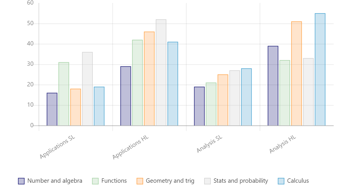
Oh, this is the big one, so I’ll cut to the chase. The most prominent differences are found in the teaching hours for each of the courses’ components, in this next table. If you can’t understand it, don’t worry, as I’ve explained it after the table.
| COMPONENT NAME | AA SL | AI SL | AA HL | AI HL |
|---|---|---|---|---|
| Number and Algebra | 19 | 16 | 39 | 29 |
| Functions | 21 | 31 | 32 | 42 |
| Geometry and Trigonometry | 25 | 18 | 51 | 46 |
| Statistics and Probability | 27 | 39 | 33 | 52 |
| Calculus | 28 | 19 | 55 | 41 |
The table shows that there are significant differences between the two courses in terms of content weightage. In essence:
Maths AA gives more emphasis on Number & Algebra, Geometry & Trigonometry and Calculus.
Maths AI gives more emphasis on Functions and Statistics & Probability.
The subject brief also describes the nature of the two courses’ syllabi:
Maths AA:
Develops important mathematical concepts in a rigorous way
Solves abstract problems as well as ones set in a meaningful context
Emphasises on construction, communication and justification of correct mathematical arguments
Teaches students to have insights into mathematical form and structure
Maths AI:
Emphasises on mathematics used in applications or mathematical modelling
Includes traditional components such as calculus and statistics
Develops strong technology skills
Encourages students to solve real world problems, construct and communicate them mathematically and interpret conclusions or generalisations
There is also a difference in their assessments.
Maths AA has one paper which prohibits the use of a calculator, Paper 1. Paper 2 and HL Paper 3 permit calculator use.Maths AI permits calculator use in all papers.
Maths AA paper 1 and paper 2 each are divided into two sections. Section A has short response questions, and Section B has extended-response questions.Maths AI paper 1 is exclusively short response questions, and paper 2 is exclusively extended response questions.
Note that HL paper 3 for both AI and AA are extended-response problem solving questions, and both of them share the same format, but have differing questions due to their differing syllabi.
Maths AA is the ‘analytical’ based, heavy on calculus and geometry/trigonometry. You cannot use a calculator in one paper. Maths AI is more ‘application’ based, heavy on functions and probability/statistics. You must use a calculator in all papers.
Which one is more useful in university?
Also one of the most common questions. Unfortunately, it is a very vague one. Neither is inherently ‘more’ useful, as it is entirely dependent on the region and your ambition in college or university.
If there is a preference for AA or AI in terms of courses, it exists for engineering or mathematics-heavy courses such as Physics or Math degrees. In these cases, AA is preferred or even required, but it only applies to countries that even differentiate between AA or AI.
I have made a very brief summary for certain popular countries for further studies and their trends for preferring AA or AI. But there exists so many exceptions that it is unjustifiable to even call it a ‘trend’ so please take this with a grain of salt and rely more on your own research.
United States: No AA/AI differentiation, but may require/prefer HL over SL for math heavy degrees
Canada: No AA/AI differentiation, but may require/prefer HL over SL for math heavy degrees
Australia: No AA/AI differentiation
United Kingdom: There are cases of differentiation in a considerable number of universities. Generally, AA HL is the course which opens the most doors, as nearly all engineering and math heavy degrees require AA HL. Many competitive economics programs even prefer or require AA HL. Of course, there are major exceptions, most notably being Oxbridge which has no preference between the two, as they already have their own entrance exams which include maths. Unfortunately, I have personally never seen any case where AI is preferred over AA, but the other way round is very common. Do correct me in the comments if you come by any exception.
So, which course should I select?
Honestly, this depends on a variety of factors. Most notably, your performance and attitude in studying mathematics, and your individual strengths or weaknesses in individual components that may lead you to choose one course or another. If you are one of those all-rounders in mathematics, then perhaps you could choose based on university plans. If you are not confident in mathematics skills but still want to pursue math-related degrees, it is also an important factor to consider.Overall, remember that you are going to spend 2 years with this subject, so make sure you like what you’re doing, and have confidence in doing well in the subject in your IB exams. Do remember to consult your teachers, school, friends and family for advice on subject selection.
So that pretty much is the end. I may have missed out certain points, maybe even have some inaccuracies, but it is the least I could do for future IB students. I hope you found this useful, and do feel free to comment with your own perspectives!
New DP mathematics courses- Syllabus
Two new courses will become part of the Diploma Programme (DP) in 2019, both taught at the Higher level (HL) and Standard level (SL). The first is Mathematics: analysis and approaches and the second is Mathematics: applications and interpretation.
From August 2019 the following courses, with first assessment in May 2021, are available:
- Mathematics: analysis and approaches SL
- Mathematics: analysis and approaches HL
- Mathematics: applications and interpretation SL
- Mathematics: applications and interpretation HL
Students can only study one course in mathematics as part of their diploma.
Each course approaches topics at varying levels of teaching hours. This guide will provide some insights into which course will be the best fit for your school and students.
The courses are separated by how they approach mathematics, described generally by the table below:
Mathematics: analysis and approaches
- Emphasis on algebraic methods
- Develop strong skills in mathematical thinking
- Real and abstract mathematical problem solving
- For students interested in mathematics, engineering physical sciences, and some economics
Mathematics: applications and interpretation
- Emphasis on modelling and statistics
- Develops strong skills in applying mathematics to the real-world
- Real mathematical problem solving using technology
- For students interested in social sciences, natural sciences, medicine, statistics, business, engineering, some economics, psychology and design
Subject breakdown
All of these courses (SL and HL in each) cover the same 5 topics within mathematics but with varying emphasis in each area: number and algebra, functions, geometry and trigonometry, statics and probability, and calculus. The chart below may help you select the right course based on the amount of time dedicated to a given topic.
Please see below the program documentation for a discussion of the math curriculum changes effective September 2019 for the IB Class of 2021.
The following chart summarizes the new courses and provides guidance in course selection:
New math course started in September 2019 for IB Class of 2021 | Course description from IB | Approximate current equivalent | Recommended prior math background |
Mathematics: Applications and interpretation | This course is designed for students who enjoy describing the real world and solving practical problems using mathematics, those who are interested in harnessing the power of technology alongside exploring mathematical models and enjoy the more practical side of mathematics. | STANDARD LEVEL (SL): This class is most similar to the current Mathematical Studies SL course. HIGHER LEVEL (HL): This course will include new content, including statistics. It is intended to meet the needs of students whose interest in mathematics is more practical than theoretical but seek more challenging content. | STANDARD LEVEL (SL): Strong Algebra 1 skills HIGHER LEVEL (HL): Strong Algebra 2 skills |
Mathematics: Analysis and approaches | This course is intended for students who wish to pursue studies in mathematics at university or subjects that have a large mathematical content; it is for students who enjoy developing mathematical arguments, problem solving and exploring real and abstract applications, with and without technology. | STANDARD LEVEL (SL): This class is most similar to the current Mathematics SL course. HIGHER LEVEL (HL): This class is most similar to the current Mathematics HL course. | STANDARD LEVEL (SL): Strong Algebra 2H skills HIGHER LEVEL (HL): Very strong Algebra 2H skills |
The following pages summarize the projected content of the new courses.
The Content
The content is still under development and items below may be subject to change when the guides are published:
Mathematics: Analysis and approaches
The number and algebra SL looks at: scientific notation, arithmetic and geometric sequences and series and their applications including financial applications, laws of logarithms and exponentials, solving exponential equations, simple proof, approximations and errors, and the binomial theorem. The number and algebra HL looks at: permutations and combinations, partial fractions, complex numbers, proof by induction, contradiction and counter–example, and solution of systems of linear equations.
The functions SL looks at: equations of straight lines, concepts and properties of functions and their graphs, including composite, inverse, the identity, rational, exponential, logarithmic and quadratic functions. So lvi n g equations both analytically and graphically, and transformation of graphs. The functions HL looks at: the factor and remainder theorems, sums and products of roots of polynomials, rational functions, odd and even functions, self–inverse functions, solving function inequalities and the modulus function.
The geometry and trigonometry SL looks at: volume and surface area of 3d solids, right angled and non –right –angled trigonometry including bearings and angles o f elevation and depression, radian measure, the unit circle and Pythagorean identity, double angle identities for sine and cosine, composite trigonometric functions, solving trigonometric equations. The geometry and trigonometry HL looks at: reciprocal trigonometric ratios, inverse trigonometric function s, compound angle identities ,double angle identity for tangent, symmetry properties of trigonometric graphs, vector theory, applications with lines and planes, and vector algebra.
The statistics and probability SL looks at: collecting data and using sampling techniques, presenting data in graphical form, measures of central tendency and spread, correlation, regression, calculating probabilities, probability diagrams, the normal distribution with standardization of variables, and the binomial distribution. The statistics and probability HL looks at: Bayes theorem, probability distributions, probability density functions, expectation algebra.
The calculus SL looks at: informal ideas of limits and convergence, differentiation including analysing graphical behaviour of functions, finding equations of normals and tangents, optimization, kinematics involving displacement, velocity, acceleration and total distance travelled, the chain, product and quotient rules, definite and indefinite integration. The calculus HL looks at: introduction to continuity and differentiability, convergence and divergence, differentiation from first principles, limits and L‘Hopital’s rule, implicit differentiation, derivatives of inverse and reciprocal trigonometric functions, integration by substitution and parts, volumes o f revolution, solution of first order differential equations using Euler‘s method, by separating variables and using the integrating factor, Maclaurin series.
Mathematics: Applications and interpretation
The number and algebra SL looks at: scientific notation, arithmetic and geometric sequences and series and their applications in finance including loan repayments, simple treatment of logarithms and exponentials, simple proof, approximations and errors. The number and algebra HL looks at: laws of logarithms, complex numbers and their practical applications, matrices and their applications for solving systems of equations, for geometric transformations, and their applications to probability.
The functions SL looks at: creating, fitting and using models with linear, exponential, natural logarithm, cubic and simple trigonometric functions. The functions HL looks at: use of log–log graphs, graph transformations, creating, fitting and using models with further trigonometric, logarithmic, rational, logistic and piecewise functions.
The geometry and trigonometry SL looks at: volume and surface area of 3d solids, right angled and non –right–angled trigonometry including bearings, surface area and volume of composite 3d solids, establishing optimum positions and paths using Voronoi diagrams.
The geometry and trigonometry HL looks at: vector concepts and their applications in kinematics, applications o f adjacency matrices, and tree and cycle algorithms.
The statistics and probability SL looks at: collecting data and using sampling techniques, presenting data in graphical form, measures of central tendency and spread, correlation using Pearson‘s pro duct–moment and Spearman’s rank correlation coefficients, regression, calculating probabilities, probability diagrams, the normal distribution, Chi–squared test for independence and goodness of fit. The statistics and probability HL looks at: the binomial and Poisson distributions, designing data collection methods, tests for reliability and validity, hypothesis testing and confidence intervals.
The calculus SL looks at: differentiation including analysing graphical behavior of functions and optimisation , using simple integration and the trapezium/ t rapezoidal rule to calculate areas of irregular shapes. The calculus HL looks at: kinematics and practical problems involving rates of change, volumes of revolution, setting up and solving models involving differential equations using numerical and analytic methods, slope fields, coupled and second–order differential equations in context.