▶️ Answer/Explanation
Part (a)
(i) Find the value of \( p \).
Total performances: \( 3 + p + 18 + 30 = 60 \)
\[ 51 + p = 60 \]
\[ p = 60 – 51 = 9 \]
(ii) Write down the modal class.
From the frequency table:
- \( 0 < n \leq 200 \): 3 performances
- \( 200 < n \leq 400 \): 9 performances
- \( 400 < n \leq 600 \): 18 performances
- \( 600 < n \leq 800 \): 30 performances
The highest frequency is 30, so the modal class is \( 600 < n \leq 800 \).
Answer: (i) \( p = 9 \), (ii) Modal class: \( 600 < n \leq 800 \)
Part (b)
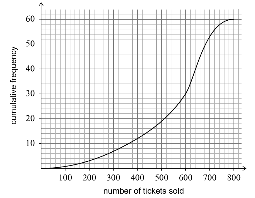
Use the cumulative frequency curve to estimate:
(i) The median number of tickets sold.
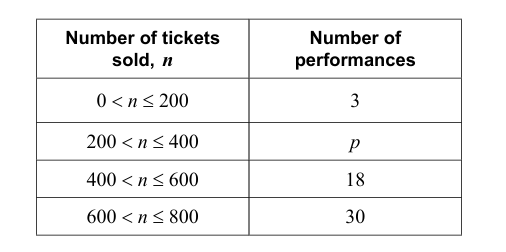
| Number of tickets sold, \( n \) | Frequency | Cumulative frequency | Midpoint (\( X_i \)) |
|---|---|---|---|
| \( 0 < n \leq 200 \) | 3 | 3 | \( \frac{0 + 200}{2} = 100 \) |
| \( 200 < n \leq 400 \) | 9 | 12 | \( \frac{200 + 400}{2} = 300 \) |
| \( 400 < n \leq 600 \) | 18 | 30 | \( \frac{400 + 600}{2} = 500 \) |
| \( 600 < n \leq 800 \) | 30 | 60 | \( \frac{600 + 800}{2} = 700 \) |
Median = average of the 30th and 31st observations: \( \frac{500 + 700}{2} = 600 \)
(ii) Number of performances where at least 80% of tickets were sold.
80% of 800 = \( 0.8 \times 800 = 640 \)
From the cumulative frequency curve, 40 performances had less than 640 tickets sold.
Thus, \( 60 – 40 = 20 \) performances had at least 640 tickets sold.
Answer: (i) Median = 600, (ii) 20 performances
Part (c)
(i) Disadvantage of surveying only the first 5%.
The sample may be biased, as the first 5% of the audience to leave may not represent the entire audience’s opinions (e.g., early leavers may have different views).
(ii) Systematic sampling method.
Select every 20th person as they leave the theatre (e.g., for 1000 attendees, 5% = 50, so \( 1000 \div 50 = 20 \)).
(iii) Sampling method for children and adults.
Quota sampling, selecting a fixed number from each subgroup (children and adults) proportional to their presence in the audience.
Answer: (i) Biased sample, (ii) Select every 20th person, (iii) Quota sampling
Part (d)
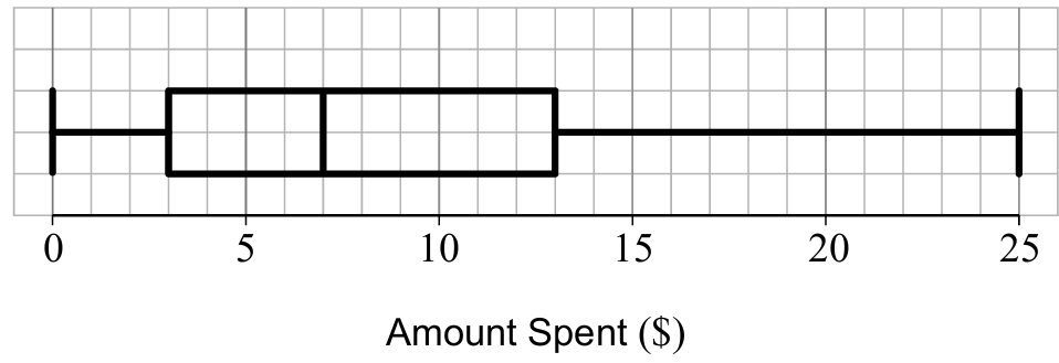
(i) Number of people who spent between $3 and $25.
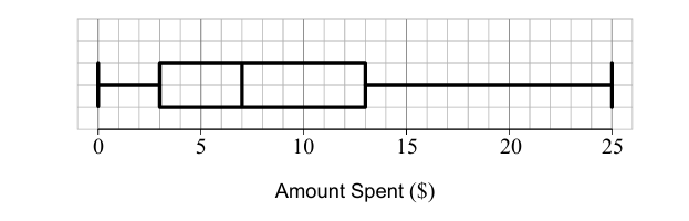
From the box and whisker diagram, 75% of the audience spent between $3 and $25.
\[ 36,000 \times 0.75 = 27,000 \]
(ii) Value of \( a \).
The median (50th percentile) from the box and whisker diagram is approximately $7.
Answer: (i) 27,000, (ii) \( a = 7 \)
Part (e)
(i) Mean number of tickets this year.
Additional tickets: \( 17 \times 60 = 1,020 \)
New total tickets: \( 36,000 + 1,020 = 37,020 \)
New mean: \( \frac{37,020}{60} = 617 \)
(ii) Effect on variance.
Adding a constant (17 tickets) to each performance shifts the mean but does not affect variance: \( \text{Var}(X + 17) = \text{Var}(X) \).
Answer: (i) Mean = 617, (ii) No effect on variance