Topic: AHL 4.14
Question
a.The random variable X represents the lifetime in hours of a battery. The lifetime may be assumed to be a continuous random variable X with a probability density function given by \(f(x) = \lambda {{\text{e}}^{ – \lambda x}}\), where \(x \geqslant 0\).
b.Find the cumulative distribution function, \(F(x)\), of X.[3]
c.Find the probability that the lifetime of a particular battery is more than twice the mean.[2]
d.Find the median of X in terms of \(\lambda \).[3]
e.Find the probability that the lifetime of a particular battery lies between the median and the mean.[2]
▶️Answer/Explanation
Markscheme
\(\int {\lambda {{\text{e}}^{ – \lambda t}}{\text{d}}t = – {{\text{e}}^{ – \lambda t}}{\text{ }}( + c)} \) A1
\( \Rightarrow F(x) = \left[ { – {{\text{e}}^{ – \lambda t}}} \right]_0^x\) (M1)
\( = 1 – {{\text{e}}^{ – \lambda t}}{\text{ }}(x \geqslant 0)\) A1
[3 marks]
\(1 – F\left( {\frac{2}{\lambda }} \right)\) M1
\( = {{\text{e}}^{ – 2}}\,\,\,\,\,( = 0.135)\) A1
[2 marks]
\(F(m) = \frac{1}{2}\) (M1)
\( \Rightarrow {{\text{e}}^{ – \lambda m}} = \frac{1}{2}\) A1
\( \Rightarrow – \lambda m = \ln \frac{1}{2}\)
\( \Rightarrow m = \frac{1}{\lambda }\ln 2\) A1
[3 marks]
\(F\left( {\frac{1}{\lambda }} \right) – F\left( {\frac{{\ln 2}}{\lambda }} \right)\) M1
\( = \frac{1}{2} – {{\text{e}}^{ – 1}}\,\,\,\,\,( = 0.132)\) A1
[2 marks]
Topic: AHL 4.14
Question
A random variable \(X\) has probability density function
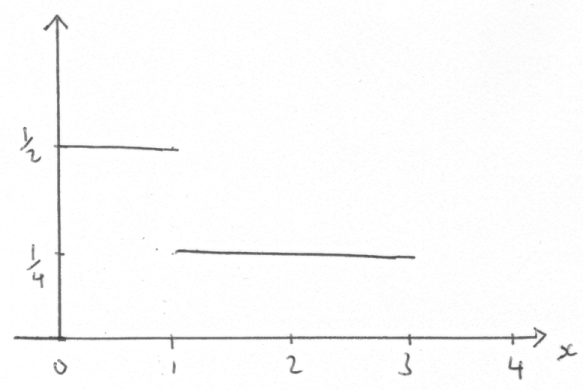
\(f(x) = \left\{ {\begin{array}{*{20}{c}} 0&{x < 0} \\ {\frac{1}{2}}&{0 \le x < 1} \\ {\frac{1}{4}}&{1 \le x < 3} \\ 0&{x \ge 3} \end{array}} \right.\)
a.Sketch the graph of \(y = f(x)\).[1]
b.Find the cumulative distribution function for \(X\).[5]
c.Find the interquartile range for \(X\).[3]
▶️Answer/Explanation
Markscheme
 A1
A1
Note: Ignore open / closed endpoints and vertical lines.
Note: Award A1 for a correct graph with scales on both axes and a clear indication of the relevant values.
[1 mark]
\(F(x) = \left\{ {\begin{array}{*{20}{c}} 0&{x < 0} \\ {\frac{x}{2}}&{0 \le x < 1} \\ {\frac{x}{4} + \frac{1}{4}}&{1 \le x < 3} \\ 1&{x \ge 3} \end{array}} \right.\)
considering the areas in their sketch or using integration (M1)
\(F(x) = 0,{\text{ }}x < 0,{\text{ }}F(x) = 1,{\text{ }}x \ge 3\) A1
\(F(x) = \frac{x}{2},{\text{ }}0 \le x < 1\) A1
\(F(x) = \frac{x}{4} + \frac{1}{4},{\text{ }}1 \le x < 3\) A1A1
Note: Accept \( < \) for \( \le \) in all places and also \( > \) for \( \ge \) first A1.
[5 marks]
\({Q_3} = 2,{\text{ }}{Q_1} = 0.5\) A1A1
\({\text{IQR is }}2 – 0.5 = 1.5\) A1
[3 marks]
Total [9 marks]
Examiners report
Part (a) was correctly answered by most candidates. Some graphs were difficult to mark because candidates drew their lines on top of the ruled lines in the answer book. Candidates should be advised not to do this. Candidates should also be aware that the command term ‘sketch’ requires relevant values to be indicated.
In (b), most candidates realised that the cumulative distribution function had to be found by integration but the limits were sometimes incorrect.
In (c), candidates who found the upper and lower quartiles correctly sometimes gave the interquartile range as \([0.5,{\text{ }}2]\). It is important for candidates to realise that that the word range has a different meaning in statistics compared with other branches of mathematics.
Topic: AHL 4.14
Question
Two independent discrete random variables \(X\) and \(Y\) have probability generating functions \(G(t)\) and \(H(t)\) respectively. Let \(Z = X + Y\) have probability generating function \(J(t)\).
a.Write down an expression for \(J(t)\) in terms of \(G(t)\) and \(H(t)\).[1]
b.By differentiating \(J(t)\), prove that
(i) \({\text{E}}(Z) = {\text{E}}(X) + {\text{E}}(Y)\);
(ii) \({\text{Var}}(Z) = {\text{Var}}(X) + {\text{Var}}(Y)\).[10]
▶️Answer/Explanation
Markscheme
\(J(t) = G(t)H(t)\) A1
[1 mark]
(i) \(J'(t) = G'(t)H(t) + G(t)H'(t)\) M1A1
\(J'(1) = G'(1)H(1) + G(1)H'(1)\) M1
\(J'(1) = G'(1) + H'(1)\) A1
so \(E(Z) = E(X) + E(Y)\) AG
(ii) \(J”(t) = G”(t)H(t) + G'(t)H'(t) + G'(t)H'(t) + G(t)H”(t)\) M1A1
\(J”(1) = G”(1)H(1) + 2G'(1)H'(1) + G(1)H”(1)\)
\( = G”(1) + 2G'(1)H'(1) + H”(1)\) A1
\({\text{Var}}(Z) = J”(1) + J'(1) – {\left( {J'(1)} \right)^2}\) M1
\( = G”(1) + 2G'(1)H'(1) + H”(1) + G'(1) + H'(1) – {\left( {G'(1) + H'(1)} \right)^2}\) A1
\( = G”(1) + G'(1) – {\left( {G'(1)} \right)^2} + H”(1) + H'(1) – {\left( {H'(1)} \right)^2}\) A1
so \({\text{Var}}(Z) = {\text{Var}}(X) + {\text{Var}}(Y)\) AG
Note: If addition is wrongly used instead of multiplication in (a) it is inappropriate to give FT apart from the second M marks in each part, as the working is too simple.
[10 marks]
Topic: AHL 4.14
Question
A continuous random variable \(T\) has a probability density function defined by
\(f(t) = \left\{ {\begin{array}{*{20}{c}} {\frac{{t(4 – {t^2})}}{4}}&{0 \leqslant t \leqslant 2} \\ {0,}&{{\text{otherwise}}} \end{array}} \right.\).
a.Find the cumulative distribution function \(F(t)\), for \(0 \leqslant t \leqslant 2\).[3]
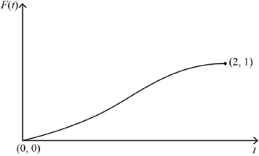
b.i.Sketch the graph of \(F(t)\) for \(0 \leqslant t \leqslant 2\), clearly indicating the coordinates of the endpoints.[2]
b.ii.Given that \(P(T < a) = 0.75\), find the value of \(a\).[2]
▶️Answer/Explanation
Markscheme
\(F(t) = \int_0^t {\left( {x – \frac{{{x^3}}}{4}} \right){\text{d}}x{\text{ }}\left( { = \int_0^t {\frac{{x(4 – {x^2})}}{4}{\text{d}}x} } \right)} \) M1
\( = \left[ {\frac{{{x^2}}}{2} – \frac{{{x^4}}}{{16}}} \right]_0^t{\text{ }}\left( { = \left[ {\frac{{{x^2}(8 – {x^2})}}{{16}}} \right]_0^t} \right){\text{ }}\left( { = \left[ {\frac{{ – 4 – {x^2}{)^2}}}{{16}}} \right]_0^t} \right)\) A1
\( = \frac{{{t^2}}}{2} – \frac{{{t^4}}}{{16}}{\text{ }}\left( { = \frac{{{t^2}(8 – {t^2})}}{{16}}} \right){\text{ }}\left( { = 1 – \frac{{{{(4 – {t^2})}^2}}}{{16}}} \right)\) A1
Note: Condone integration involving \(t\) only.
Note: Award M1A0A0 for integration without limits eg, \(\int {\frac{{t(4 – {t^2})}}{4}{\text{d}}t = \frac{{{t^2}}}{2} – \frac{{{t^4}}}{{16}}} \) or equivalent.
Note: But allow integration \( + \) \(C\) then showing \(C = 0\) or even integration without \(C\) if \(F(0) = 0\) or \(F(2) = 1\) is confirmed.
[3 marks]

correct shape including correct concavity A1
clearly indicating starts at origin and ends at \((2,{\text{ }}1)\) A1
Note: Condone the absence of \((0,{\text{ }}0)\).
Note: Accept 2 on the \(x\)-axis and 1 on the \(y\)-axis correctly placed.
[2 marks]
attempt to solve \(\frac{{{a^2}}}{2} – \frac{{{a^4}}}{{16}} = 0.75\) (or equivalent) for \(a\) (M1)
\(a = 1.41{\text{ }}( = \sqrt 2 )\) A1
Note: Accept any answer that rounds to 1.4.
[2 marks]
Topic: AHL 4.14
Question
Consider an unbiased tetrahedral (four-sided) die with faces labelled 1, 2, 3 and 4 respectively.
The random variable X represents the number of throws required to obtain a 1.
a.State the distribution of X.[1]
b.Show that the probability generating function, \(G\left( t \right)\), for X is given by \(G\left( t \right) = \frac{t}{{4 – 3t}}\).[4]
c.Find \(G’\left( t \right)\).[2]
d.Determine the mean number of throws required to obtain a 1.[1]
▶️Answer/Explanation
Markscheme
X is geometric (or negative binomial) A1
[1 mark]
\(G\left( t \right) = \frac{1}{4}t + \frac{1}{4}\left( {\frac{3}{4}} \right){t^2} + \frac{1}{4}{\left( {\frac{3}{4}} \right)^2}{t^3} + \ldots \) M1A1
recognition of GP \(\left( {{u_1} = \frac{1}{4}t,\,\,r = \frac{3}{4}t} \right)\) (M1)
\( = \frac{{\frac{1}{4}t}}{{1 – \frac{3}{4}t}}\) A1
leading to \(G\left( t \right) = \frac{t}{{4 – 3t}}\) AG
[4 marks]
attempt to use product or quotient rule M1
\(G’\left( t \right) = \frac{4}{{{{\left( {4 – 3t} \right)}^2}}}\) A1
[2 marks]
4 A1
Note: Award A1FT to a candidate that correctly calculates the value of \(G’\left( 1 \right)\) from their \(G’\left( t \right)\).
[1 mark]
