Question
Daniel grows apples and chooses at random a sample of 100 apples from his harvest.
He measures the diameters of the apples to the nearest cm. The following table shows the distribution of the diameters.
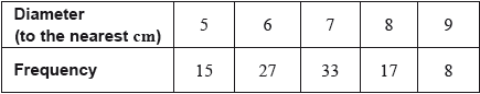
Using your graphic display calculator, write down the value of
(i) the mean of the diameters in this sample;
(ii) the standard deviation of the diameters in this sample.[3]
Daniel assumes that the diameters of all of the apples from his harvest are normally distributed with a mean of 7 cm and a standard deviation of 1.2 cm. He classifies the apples according to their diameters as shown in the following table.

Calculate the percentage of small apples in Daniel’s harvest.[3]
Daniel assumes that the diameters of all of the apples from his harvest are normally distributed with a mean of 7 cm and a standard deviation of 1.2 cm. He classifies the apples according to their diameters as shown in the following table.
Of the apples harvested, 5% are large apples.
Find the value of \(a\).[2]
Daniel assumes that the diameters of all of the apples from his harvest are normally distributed with a mean of 7 cm and a standard deviation of 1.2 cm. He classifies the apples according to their diameters as shown in the following table.
Find the percentage of medium apples.[2]
Daniel assumes that the diameters of all of the apples from his harvest are normally distributed with a mean of 7 cm and a standard deviation of 1.2 cm. He classifies the apples according to their diameters as shown in the following table.
This year, Daniel estimates that he will grow \({\text{100}}\,{\text{000}}\) apples.
Estimate the number of large apples that Daniel will grow this year.[2]
Answer/Explanation
Markscheme
(i) \(6.76{\text{ (cm)}}\) (G2)
Notes: Award (M1) for an attempt to use the formula for the mean with a least two rows from the table.
(ii) \(1.14{\text{ (cm)}}\;\;\;\left( {1.14122 \ldots {\text{ (cm)}}} \right)\) (G1)
\({\text{P}}({\text{diameter}} < 6.5) = 0.338\;\;\;(0.338461)\) (M1)(A1)
Notes: Award (M1) for attempting to use the normal distribution to find the probability or for correct region indicated on labelled diagram. Award (A1) for correct probability.
\(33.8(\% )\) (A1)(ft)(G3)
Notes: Award (A1)(ft) for converting their probability into a percentage.
\({\text{P}}({\text{diameter}} \geqslant a) = 0.05\) (M1)
Note: Award (M1) for attempting to use the normal distribution to find the probability or for correct region indicated on labelled diagram.
\(a = 8.97{\text{ (cm)}}\;\;\;(8.97382 \ldots )\) (A1)(G2)
\(100 – (5 + 33.8461 \ldots )\) (M1)
Note: Award (M1) for subtracting “\(5+\) their part (b)” from 100 or (M1) for attempting to use the normal distribution to find the probability \({\text{P}}\left( {6.5 \leqslant {\text{diameter}} < {\text{their part (c)}}} \right)\) or for correct region indicated on labelled diagram.
\( = 61.2(\% )\;\;\;\left( {61.1538 \ldots (\% )} \right)\) (A1)(ft)(G2)
Notes: Follow through from their answer to part (b). Percentage symbol is not required. Accept \(61.1(\%)\) (\(61.1209\ldots(\%)\)) if \(8.97\) used.
\(100\,000 \times 0.05\) (M1)
Note: Award (M1) for multiplying by \(0.05\) (or \(5\%\)).
\( = 5000\) (A1)(G2)
Question
On one day 180 flights arrived at a particular airport. The distance travelled and the arrival status for each incoming flight was recorded. The flight was then classified as on time, slightly delayed, or heavily delayed.
The results are shown in the following table.

A χ2 test is carried out at the 10 % significance level to determine whether the arrival status of incoming flights is independent of the distance travelled.
The critical value for this test is 7.779.
A flight is chosen at random from the 180 recorded flights.
State the alternative hypothesis.[1]
Calculate the expected frequency of flights travelling at most 500 km and arriving slightly delayed.[2]
Write down the number of degrees of freedom.[1]
Write down the χ2 statistic.[2]
Write down the associated p-value.[1]
State, with a reason, whether you would reject the null hypothesis.[2]
Write down the probability that this flight arrived on time.[2]
Given that this flight was not heavily delayed, find the probability that it travelled between 500 km and 5000 km.[2]
Two flights are chosen at random from those which were slightly delayed.
Find the probability that each of these flights travelled at least 5000 km.[3]
Answer/Explanation
Markscheme
The arrival status is dependent on the distance travelled by the incoming flight (A1)
Note: Accept “associated” or “not independent”.[1 mark]
\(\frac{{60 \times 45}}{{180}}\) OR \(\frac{{60}}{{180}} \times \frac{{45}}{{180}} \times 180\) (M1)
Note: Award (M1) for correct substitution into expected value formula.
= 15 (A1) (G2)[2 marks]
4 (A1)
Note: Award (A0) if “2 + 2 = 4” is seen.[1 mark]
9.55 (9.54671…) (G2)
Note: Award (G1) for an answer of 9.54.[2 marks]
0.0488 (0.0487961…) (G1)[1 mark]
Reject the Null Hypothesis (A1)(ft)
Note: Follow through from their hypothesis in part (a).
9.55 (9.54671…) > 7.779 (R1)(ft)
OR
0.0488 (0.0487961…) < 0.1 (R1)(ft)
Note: Do not award (A1)(ft)(R0)(ft). Follow through from part (d). Award (R1)(ft) for a correct comparison, (A1)(ft) for a consistent conclusion with the answers to parts (a) and (d). Award (R1)(ft) for χ2calc > χ2crit , provided the calculated value is explicitly seen in part (d)(i).[2 marks]
\(\frac{{52}}{{180}}\,\,\left( {0.289,\,\,\frac{{13}}{{45}},\,\,28.9\,{\text{% }}} \right)\) (A1)(A1) (G2)
Note: Award (A1) for correct numerator, (A1) for correct denominator.[2 marks]
\(\frac{{35}}{{97}}\,\,\left( {0.361,\,\,36.1\,{\text{% }}} \right)\) (A1)(A1) (G2)
Note: Award (A1) for correct numerator, (A1) for correct denominator.[2 marks]
\(\frac{{14}}{{45}} \times \frac{{13}}{{44}}\) (A1)(M1)
Note: Award (A1) for two correct fractions and (M1) for multiplying their two fractions.
\( = \frac{{182}}{{1980}}\,\,\left( {0.0919,\,\,\frac{{91}}{{990}},\,0.091919 \ldots ,\,9.19\,{\text{% }}} \right)\) (A1) (G2)[3 marks]
Question
The lengths (\(l\)) in centimetres of \(100\) copper pipes at a local building supplier were measured. The results are listed in the table below.

Write down the mode.[1]
Using your graphic display calculator, write down the value of
(i) the mean;
(ii) the standard deviation;
(iii) the median.[4]
Find the interquartile range.[2]
Draw a box and whisker diagram for this data, on graph paper, using a scale of \(1{\text{ cm}}\) to represent \(5{\text{ cm}}\).[4]
Sam estimated the value of the mean of the measured lengths to be \(43{\text{ cm}}\).
Find the percentage error of Sam’s estimated mean.[2]
Answer/Explanation
Markscheme
\(47.5{\text{ (cm)}}\) (A1)
(i) \(45.85{\text{ (cm)}}\) (G2)
Note: Accept \(45.9\) .
(ii) \(17.1{\text{ }}(17.0888 \ldots )\) (G1)
(iii) \(47.5{\text{ (cm)}}\) (G1)
\(62.5 – 32.5 = 30\) (M1)(A1)(G2)
Note: Award (M1) for correct quartiles seen.

(A1) for correct label and scale
(A1)(ft) for correct median
(A1)(ft) for correct quartiles and box
(A1) for endpoints at \(17.5\) and \(77.5\) joined to box by straight lines (A1)(A1)(ft)(A1)(ft)(A1)
Notes: The final (A1) is lost if the lines go through the box. Follow through from their parts (b) and (c).
\(\varepsilon = \left| {\frac{{43 – 45.85}}{{45.85}}} \right| \times 100\% \) (M1)
Note: Award (M1) for their correct substitution in \(\% \) error formula.
\( = 6.22\% \) (\(6.21592 \ldots \)) (A1)(ft)(G2)
Notes: Follow through from their answer to part (b)(i). Accept \(6.32\% \) with use of \(45.9\) .