Question
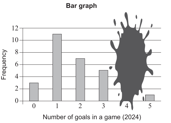
For a \( 2024 \) soccer tournament, Andrew has compiled a bar chart showing the total number of goals scored in every match. However, the vertical bar representing the frequency of matches with exactly \( 4 \) goals is currently illegible. Andrew uses the information from this chart to begin constructing a frequency table.
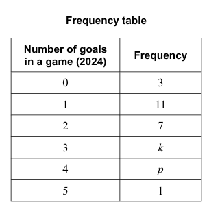
(a) Determine the value of \( k \) as shown in the frequency table.
(b) Andrew notes that the average (mean) number of goals scored per game throughout the entire tournament was \( 2.2 \).
(i) Formulate an equation for the mean in terms of the unknown frequency \( p \).
(ii) Solve the equation to find the value of \( p \).
The distribution of goals per match for the subsequent \( 2025 \) soccer tournament is presented in the box and whisker plot below.
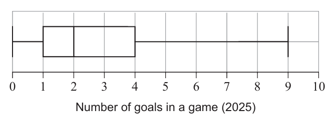
(c) By analyzing the \( 2025 \) box plot alongside the \( 2024 \) frequency data, Andrew suggests that the goal distributions for both years are remarkably similar. Support this claim by providing two specific observations, comparing any two of the following: range, symmetry, median, or interquartile range (IQR). Ensure you include numerical values in your comparisons.
(d) Andrew randomly selects one match from the \( 2024 \) data. Let event \( F \) be defined as “the match had either \( 0 \) or \( 1 \) goal scored”. Identify which event(s) from the following list are equivalent to the complement of \( F \) (denoted as \( F’ \)).
| Event | Description |
|---|---|
| \( A \) | Exactly \( 2 \) goals were scored in this match. |
| \( B \) | More than \( 1 \) goal was scored in this match. |
| \( C \) | At least \( 2 \) goals were scored in this match. |
| \( D \) | Either \( 0 \) or \( 1 \) goal was scored in every match except this one. |
| \( E \) | Neither \( 0 \) nor \( 1 \) goal was scored in any match. |
(e) If it is known that exactly \( 1 \) goal was scored in the first match Andrew watches, calculate the probability that exactly \( 1 \) goal was also scored in the second match he watches. State your answer as a simplified fraction.
(f) Determine the probability that exactly \( 5 \) goals were scored in the first match Andrew watches, followed by exactly \( 0 \) goals in the second match he watches.
Most-appropriate topic codes (IB Mathematics AI SL 2025):
• SL 4.3: Mean and measures of dispersion — part (b), (c)
• SL 4.5: Probability of an event and its complement — part (d)
• SL 4.6: Conditional probability and combined events without replacement — parts (e), (f)
▶️ Answer/Explanation
(a)
From the bar graph, the frequency for \( 3 \) goals is \( 5 \).
\(\boxed{5}\)
(b)(i)
Total number of games: \( 3 + 11 + 7 + 5 + p + 1 = 27 + p \)
Sum of goals: \( 0 \times 3 + 1 \times 11 + 2 \times 7 + 3 \times 5 + 4p + 5 \times 1 = 45 + 4p \)
Mean: \( \frac{45 + 4p}{27 + p} = 2.2 \)
Equation: \(\boxed{\frac{45+4p}{27+p}=2.2}\)
(b)(ii)
Solving: \( 45 + 4p = 2.2(27 + p) \)
\( 45 + 4p = 59.4 + 2.2p \)
\( 1.8p = 14.4 \)
\( p = 8 \)
\(\boxed{8}\)
(c)
From \( 2024 \) data:
• Median \( = 2 \)
• \( Q_1 = 1 \), \( Q_3 = 4 \rightarrow \text{IQR} = 3 \)
• Range \( = 5 \)
From \( 2025 \) box plot:
• Median \( = 2 \)
• \( Q_1 = 1 \), \( Q_3 = 4 \rightarrow \text{IQR} = 3 \)
• Range \( = 5 \)
Two valid comparisons:
\( 1. \) Both distributions have the same median (\( 2 \)).
\( 2. \) Both have the same interquartile range (\( 3 \)).
Scoring: Any two correct comparisons using values.
(d)
\( F \): scoring \( 0 \) or \( 1 \) goal \( \rightarrow F’ \): scoring not \( 0 \) and not \( 1 \) goal \( \rightarrow \) scoring \( \geq 2 \) goals.
This matches:
• \( B \): Scoring more than \( 1 \) goal
• \( C \): Scoring at least \( 2 \) goals
\(\boxed{B \text{ and } C}\)
(e)
After \( 1 \) goal in first game, remaining games \( = 34 \), frequency of \( 1 \) goal left \( = 11 – 1 = 10 \).
Probability \( = \frac{10}{34} = \frac{5}{17} \).
\(\boxed{\frac{5}{17}}\)
(f)
Total games initially \( = 35 \).
\( P(\text{5 goals first}) = \frac{1}{35} \)
After, games left \( = 34 \), \( 0 \)-goal games left \( = 3 \).
\( P(\text{0 goals second}) = \frac{3}{34} \)
Multiply: \( \frac{1}{35} \times \frac{3}{34} = \frac{3}{1190} \).
\(\boxed{\frac{3}{1190}}\) (\( \approx 0.00252 \))