AP Statistics- Unit 4: Probability, Random Variables, and Probability Distributions Summary Notes

Probability, Random Variables, and Probability Distributions
On your AP Statistics exam, 10‒20% of questions will cover the topic of Probability, Random Variables, and Probability Distributions.

Basic Probability
The field of probability involves random processes. That is, processes whose results are determined by chance. The set of all possible outcomes is called the sample space, and an event is any subset of the sample space.

The probability of an event is the likelihood of it occurring and is represented as a number between 0 and 1 , inclusive. If the chance process is repeatable, the probability can be interpreted as the relative frequency with which the event will occur if the process is repeated many times.

If all of the outcomes in the sample space are equally like to occur, then the probability of an event \(E\) is the ratio of the number of outcomes in \(E\) to the number of outcomes in the sample space.

The completement of an event \(\mathrm{E}\), denoted \(\mathrm{E}^{\prime}\) or \(\mathrm{E}^{\mathrm{c}}\), is the event that consists of all outcomes that are not in \(\mathrm{E}\).

In many real-world situations, probabilities can be very difficult to calculate. When this happens, simulation can be used. Simulation is a technique in which random events are simulated in a way that matches as closely as possible the random process that gives rise to the probability. This is usually done by generating random numbers. The simulation can be repeated many times, and the simulated outcome examined for each repetition. The relative frequency of an event in this sequence of simulated outcomes is an estimate of the probability of the event.

Joint and Conditional Probability
When a probability involves two events both occurring, it is referred to as a joint probability. The joint event is denoted using a \(\cap\), as in \(A \cap B\).

Sometimes we are interested in a probability that depends on knowledge about whether or not another event occurred. This is called a conditional probability. The probability that an \(A\) will occur given that another event \(B\) is known to have occurred is denoted \(P(A \mid B)\), and its value is given by \(P(A \mid B)=\frac{P(A \cap B)}{P(B)}\).

Rearranging the terms in this formula, we get the multiplication rule for joint probabilities: \(P(A \cap B)=P(A) \cdot P(B \mid A)\).

If \(P(A \mid B)=P(A)\), then events \(A\) and \(B\) are said to be independent. The significance of independence is that whether or not one of the events occur has no influence on the probability of the other event. The roles of \(A\) and \(B\) can always be switched, so that \(P(B \mid A)=\) \(P(B)\) will also be true if \(A\) and \(B\) are independent. Another important consequence of independence is that the multiplication rule simplifies to \(P(A \cap B)=P(A) \cdot P(B)\). This last equation can also be used to check for independence.

Unions and Mutually Exclusive Events
The event consisting of either \(A\) or \(B\) occurring is called a union, and is denoted by \(A \cup B\). Its probability is given by the addition rule: \(P(A \cup B)=P(A)+P(B)-P(A \cap B)\). Note that this is inclusive, so that any outcomes that are in both \(\mathrm{A}\) and \(\mathrm{B}\) are included in \(A \cup B\).

Two events are called mutually exclusive if they cannot both occur, so that their joint probability is 0 . In other words, \(A\) and \(B\) are mutually exclusive if \(P(A \cap B)=0\). When this occurs, the last term in the addition rule given previously is 0 . Therefore, if \(\mathrm{A}\) and \(\mathrm{B}\) are mutually exclusive, the addition rule simplifies to \(P(A \cup B)=P(A)+P(B)\).

Free Response Tip
Do not assume events are mutually exclusive unless you are sure they really are! There is no downside to using the full addition rule. If it happens that they are mutually exclusive, the last term will simply not contribute to the probability.

Random Variables and Probability Distributions
A random variable is a variable whose numerical value depends on the outcome of a random experiment, so that it takes on different values with certain probabilities. A random variable is called discrete if it can take on finitely or countably many values. The sum of the probabilities of the possible values is always equal to 1 , since they represent all possible outcomes of the experiment.

A probability distribution represents the possible values of a random variable along with their respective probabilities. It is often represented as a table or graph, as in the following example:

The table shows a random variable \(X\) that can take on each of the values \(1,2,3,4\), and 5. It takes on the value 1 with probability 0.2 , the value 2 with probability 0.3 , and so on. Note that the sum of the probabilities is \(0.2+0.3+0.1+0.25+0.15=1\), as expected. The notation \(P(X=x)\) in the second row represents the probability of the random variable \((X)\) taking on one of its possible values \((x)\).

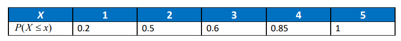
Sometimes it is beneficial to have a cumulative probability distribution, which shows the probabilities of all values of a random variable less than or equal to a given value.
The cumulative distribution for the example in the previous table is as follows:

A probability distribution has a mean and a standard deviation, just like a population. The mean, or expected value, of a discrete random variable \(\mathrm{X}\) is \(\mu_X=\sum x_i \cdot P\left(x_i\right)\). Its standard deviation is \(\sigma_X=\sqrt{\sum\left(x_i-\mu_X\right)^2 \cdot P\left(x_i\right)}\).

Combining Random Variables
If \(X\) and \(Y\) are two discrete random variables, a new random variable can be constructed by combining \(X\) and \(Y\) in a linear combination \(a X+b Y\), where \(a\) and \(b\) are any real numbers. The

mean of this new random variable is \(\mu_{a X+b Y}=a \mu_X+b \mu_Y\). If the two variables are independent, so that information obtained about one of them does not affect the distribution of the other, then the standard deviation of the linear combination is \(\sigma_{a X+b Y}=\sqrt{a^2 \sigma_Y^2+b^2 \sigma_Y^2}\). If the variables are not independent, the computation of the standard deviation of the linear combination is well beyond the scope of AP Statistics.

A single random variable can also be transformed into a new one by means of the linear equation \(Y=a+b X\). The mean of the transformed variable is \(\mu_Y=a+b \mu_X\), and its standard deviation is \(\sigma_Y=|b| \sigma_X\). In addition, if \(a\) and \(b\) are both positive, then the distribution of \(Y\) has the same shape as the distribution of \(X\).

Binomial and Geometric Distributions
A Bernoulli trial is an experiment that satisfies the following conditions:

  • There are only two possible outcomes, called success and failure
  •  The probability of success is the same every time the experiment is conducted

We will let \(p\) denote the probability of success. Because failure is the complement of success, the probability of failure is then \(1-p\).

Consider repeating a Bernoulli trial \(n\) times and counting the number of successes that occur in these repetitions. If we call the number of successes \(X\), then \(X\) is called a binomial random variable. The probability of exactly \(x\) successes in \(n\) trials is given by \(P(X=x)=\left(\begin{array}{l}n \\ x\end{array}\right) p^x(1-p)^{n-x}\) Here \(\left(\begin{array}{l}n \\ x\end{array}\right)\) is the binomial coefficient often referred to as a combination. Its value is \(\left(\begin{array}{l}n \\ x\end{array}\right)=\frac{n !}{x !(n-x) !}\).

The mean of a binomial random variable is \(\mu_X=n p\), and its standard deviation is \(\sigma_X=\sqrt{n p(1-p)}\).

A geometric random variable is also related to Bernoulli trials. Unlike a binomial random variable, a geometric random variable \(X\) is the number of the trial on which a success first occurs. The value is given by \(P(X=x)=(1-p)^{1-x} p\). Its mean is \(\mu_X=\frac{1}{p}\) and its standard deviation is \(\sigma_X=\frac{\sqrt{1-p}}{p}\).

Free Response Tip
Be careful to not get confused by the terms success and failure in the description of binomial and geometric distribution. They do not necessarily have any bearing on success and failure as the words might generally be applied in any given situation. For example, if a problem involves counting the number of phones in a case of 20 produced in a factory, it would be advantageous to refer to a phone being defective as a success, even though it is certainly not that from the perspective of the manufacturer!

Suggested Reading

  •  Starnes \& Tabor. The Practice of Statistics. \(6^{\text {th }}\) edition. Chapters 5 and 6. New York, NY: Macmillan.
  • Larson \& Farber. Elementary Statistics: Picturing the World. \(7^{\text {th }}\) edition. Chapters 3 and 4. New York, NY: Pearson.
  • Bock, Velleman, De Veaux, \& Bullard. Stats:Modeling the World. \(5^{\text {th }}\) edition. Chapters 13-16. New York, NY: Pearson.
  •  Sullivan. Statistics: Informed Decisions Using Data. \(5^{\text {th }}\) edition. Chapters 5 and 6. New York, NY: Pearson.
  • Peck, Short, \& Olsen. Introduction to Statistics and Data Analysis. \(6^{\text {th }}\) edition. Chapters 6 and 7. Boston, MA: Cengage Learning.

Sample Probability, Random Variables, and Probability Distributions Questions

The probability that Valley Creek will flood in any given year has been estimated from 150 years of historical data to be 0.20 . Which of the following is an accurate interpretation of this statement?
A. Valley Creek will flood once every five years.
B. In the next 50 years, Valley Creek will flood about in about 10 of those years.
C. In the next 100 years, Valley Creek cannot flood fewer than 20 times.
D. In the last 50 years, Valley Creek flooded exactly 10 times.
E. In the next 50 years, Valley Creek will flood exactly 10 times.

▶️Answer/Explanation

Explanation:
The correct answer is B. In the long run, this statement means that Valley Creek floods about \(20 \%\) of the time. Since \(20 \%\) of 50 is 10 , we expect it to flood about 10 times. The statement in choice A is probabilistic; it does not literally imply that the creek will necessarily flood every fifth year, but rather of the past 150 years, it has flood 30 times. Choices \(C\) and \(E\) are also incorrect because it does not literally imply that the creek will necessarily flood every fifth year; in the long run, Valley Creek floods \(20 \%\) of the time, not necessarily exactly \(20 \%\) of the time. Choice \(D\) is incorrect because the past 150 years were used to formulate this probabilistic statement. It could be the case that Valley Creek flooded 30 times in the first 100 years and never thereafter.

The probability that a visitor of the local botanical gardens walks through the rose garden is 0.65 , and the probability that a visitor meanders through the new meadow is 0.45 . The probability that a visitor does both activities on the same day is 0.32 . What is the probability that a visitor does at least one of the activities on a given day?
A. 0
B. 0.2925
C. 0.78
D. 0.22

E. 0.50

▶️Answer/Explanation

Explanation:
The correct answer is \(\mathrm{C}\). Let \(A\) be the event “walks through the rose garden” and \(B\) the event “meanders through the new meadow.” We must compute \(P(A \cup B)\). To do so, use the addition formula, as follows:
$
\begin{aligned}
& P(A \cup B)=P(A)+P(B)-P(A \cap B) \\
& =0.65+0.45-0.32=0.78
\end{aligned}
$

Choice A is incorrect because this event is far from impossible. Use the addition formula to compute the probability of the event “walks through rose garden OR meanders through new meadow.” Choice B is incorrect because when computing \(P(A \cup B)\), you multiplied the probabilities \(P(A)\) and \(P(B)\), which is incorrect; you must use the addition formula. Choice \(D\) is incorrect because this is the probability that a visitor does neither of these two activities on a given day. Choice \(\mathrm{E}\) is incorrect because there is not a 50-50 chance of this event occurring. You must use the addition formula to compute the probability of the event “walks through rose garden OR meanders through new meadow.”

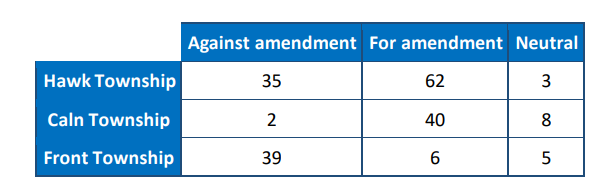
To study the relationship between township and support for a certain amendment concerning property tax, 200 registered voters were surveyed with the following results:

What percentage of those surveyed were against the amendment and were residents of Front Township?
A. \(80.5 \%\)

B. \(51.3 \%\)

C. \(78 \%\)

D. \(19.5 \%\)

E. \(39 \%\)

▶️Answer/Explanation

Explanation:
The correct answer is D. The event of interest is “against amendment AND lives in Front Township.” The number of respondents satisfying this criterion is in the lower left cell of the table. Hence, the percentage satisfying this criterion is \(39 / 200=19.5 \%\). Choice A is the percentage of those sampled that satisfies neither condition. Choice B is incorrect because you computed a conditional probability assuming “against amendment” as given information. As the problem is stated, you are looking for the probability of an “AND” event. Choice C is incorrect because you computed a conditional probability assuming “lived in Front Township” as given information. As the problem is stated, you are looking for the probability of an “AND” event. Choice \(\mathrm{E}\) is incorrect because this is the number of respondents satisfying the criterion, not the percentage. You must divide this by the total sample size, 200.

Scroll to Top