AP Statistics- Unit 5: Sampling Distributions Summary Notes

Sampling Distributions

About \(7-12 \%\) of the questions on your exam will cover the topic of Sampling Distributions.

The Normal Distribution
Unlike a discrete random variable, a continuous random variable can take on any value within some set. Instead of probabilities being associated with individual values of the variable, probabilitiesare assigned to every possible interval of values. The most important type of continuous random variable is a normal random variable.
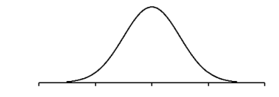
A normal distribution has a shape that is often described as a bell-shaped curve. It is unimodal and symmetric:

The probability associated with any given interval is given by the area under the normal curve over that interval. The intervals are generally one of four types:

  •  \(X<a\). This is called a left-tailed interval. If the probability associated with it is \(P(X<a)=\frac{p}{100}\), this means that the smallest \(p \%\) of values in the population are less than \(a\).
  • \(X>a\). This is called a right-tailed interval. If the probability associated with it is \(P(X>a)=\frac{p}{100}\), this means that the largest \(p \%\) of values in the population are greater than \(a\).
  •  \(|X|>a\), where \(a>0\). This is a two-tailed interval. If the probability associated with it is \(P(|X|>a)=\frac{p}{100}\), this means that the largest \(\frac{p}{2} \%\) of values are greater than \(a\), and the smallest \(\frac{p}{2} \%\) of values are less than \(-a\).
  •  \(a<X<b\). If the probability associated with this interval is \(P(a<X<B)=\frac{p}{100}\), this means that \(p \%\) of the values are between \(a\) and \(b\).

As mentioned previously, a normal distribution is defined by two parameters: its mean, \(\mu\), and its standard deviation, \(\sigma\). Every combination of \(\mu\) and \(\sigma\) determine a different normal distribution. The standard normal distribution is the normal distribution with \(\mu=0\) and \(\sigma=1\).

Areas under any normal curve can be found using a calculator or computer software. There are also standard normal tables in many textbooks that can be used to find the probabilities of the standard normal distribution. Using z-scores, however, the probabilities in any normal distribution can be made equivalent to the probabilities in a standard normal distribution. First, find the \(z\)-score(s) of the endpoint(s) of the interval of interest. Then simply use the standard normal distribution to find the probability of the new interval. This probability is also the correct value for the original interval.

Central Limit Theorem
Consider a statistic of interest, such as a mean, median, standard deviation, or proportion of a large population. Now take all possible samples of a given size from within this population and calculate the statistic for each sample. The resulting values would themselves form a distribution. This distribution is called the sampling distribution of the statistic.

The Central Limit Theorem is the most important tool needed in doing inferential statistics. It states that under certain assumptions, the sampling distribution of the mean will be approximately normally distributed. One requirement is that either the o riginal population itself be normally distributed, or that the sample size be at least 30 . In addition, the samples must be independent of each other.

Since we are going to use sampling distributions to infer parameters of the population, it is important to know when this will give accurate values. A statistic is an unbiased estimator of its corresponding parameter if the mean of its sampling distribution is equal to the parameter. For example, sample mean is an unbiased estimator, while sample standard deviation is not.

Sampling Distribution for Proportions
Consider a population for which we are interested in the proportion that satisfy some condition. This means there is a categorical variable, and that we want to know the proportion

\(p\) of values that are in a certain category. The sample proportions \(\hat{p}\) from all independent samples of size \(n\) form a sampling distribution with mean \(\mu_{\hat{p}}=p\) and standard deviation \(\sigma_{\hat{p}}=\sqrt{\frac{p(1-p)}{n}}\). If the samples are not independent, then the standard deviation is not as given; however, if the sample size \(n\) is less than \(10 \%\) of the population size, it is very close to accurate. If \(n p \geq 10\) and \(n(1-p) \geq 10\), the sampling distribution is approximately normal.

If we are not interested in a single population proportion, but rather in the difference between two proportions \(p_1\) and \(p_2\), from populations with samples of sizes \(n_1\) and \(n_2\), the distribution is given by \(\mu_{\hat{p}_1-\hat{p}_2}=p_1-p_2\) and \(\mu_{\hat{p}_1-\hat{p}_2}=\sqrt{\frac{p_1\left(1-p_1\right)}{n_1}+\frac{p_2\left(1-p_2\right)}{n_2}}\). Here again, if the samples are not independent the standard deviation is not quite correct, but it is very close if the sample sizes are less than \(10 \%\) of the population sizes. If \(n_1 p_1, n_1\left(1-p_1\right), n_2 p_2\), and \(n_2\left(1-p_2\right)\) are all at least 10 , the sampling distribution of \(\hat{p}_1-\hat{p}_2\) is approximately normal.

Sampling Distribution for Means
The sampling distribution of sample means is also easy to describe. If independent samples of size \(n\) are taken from a population with mean \(\mu\) and standard deviation \(\sigma\), then the sampling distribution has \(\mu_{\bar{x}}=\mu\) and \(\sigma_{\bar{x}}=\frac{\sigma}{\sqrt{n}}\). Even in dependent samples, the standard deviation is accurate if the sample size is less than \(10 \%\) of the population. The sampling distribution is approximately normal if either the population itself is approximately normal or if \(n \geq 30\).

If samples of sizes \(n_1\) and \(n_2\) are taken from two independent populations with means \(\mu_1\) and \(\mu_2\) and standard deviations \(\sigma_1\) and \(\sigma_2\), the sampling distribution of \(\bar{x}_1-\bar{x}_2\) has mean \(\mu_{\bar{x}_1-\bar{x}_2}=\mu_1-\mu_2\) and standard deviation \(\sigma_{\bar{x}_1-\bar{x}_2}=\sqrt{\frac{\sigma_1^2}{n_1}+\frac{\sigma_2^2}{n_2}}\). There are similar conditions here as well: the standard deviation given is accurate even for dependent samples if the sample sizes are less than \(10 \%\) of their respective populations, and the sampling distribution is approximately normal if either the two populations are approximately normal or if \(n_1\) and \(n_2\) are both at least 30 .

Suggested Reading

  • Starnes \& Tabor. The Practice of Statistics. \(6^{\text {th }}\) edition. Chapter 7. New York, NY: Macmillan.
  •  Larson \& Farber. Elementary Statistics: Picturing the World. \(7^{\text {th }}\) edition. Chapter 5. New York, NY: Pearson.
  •  Bock, Velleman, De Veaux, \& Bullard. Stats:Modeling the World. \(5^{\text {th }}\) edition. Chapter 17. New York, NY: Pearson.
  •  Sullivan. Statistics: Informed Decisions Using Data. \(5^{\text {th }}\) edition. Chapters 7 and 8. New York, NY: Pearson.
  •  Peck, Short, \& Olsen. Introduction to Statistics and Data Analysis. \(6^{\text {th }}\) edition. Chapter 8. Boston, MA: Cengage Learning.

Sample Sampling Distributions Questions

Which of the following statements is (are) true?
I. The larger the sample, the smaller the variance of the sampling distribution.
II. Sampling distributions from non-normal populations are approximately normal when the sample size is large.
III. If the population size is much larger than the sample size, then the variance of the sampling distribution remains unchanged, no matter what the sample size is.
A.I only
B. III only
C. I and II only
D. I and III only
E. I, II, and III

▶️Answer/Explanation

Explanation:
The correct answer is C. Statement I is true because the variance of the sampling distribution is \(\frac{\sigma^2}{n}\), where \(n\) is the sample size. So, as \(n\) increases, this fraction decreases. Statement II is true because it is a direct consequence of the Central Limit Theorem.

Which of the following is a consequence of the Central Limit Theorem for a sample size \(n\) ?
A. A standard deviation of the sample mean random variable is greater than the population standard deviation.
B. The expectation of the sample mean random variable is equal to the population mean \(\mu\) when \(n\) is large.
C. The sampling distribution of the sample mean is always normal for any sample size \(n\).
D. The standard deviation of the set of sample mean random variable is equal to the population standard deviation \(\sigma\).
E. mean of the sample mean random variable is always less than the mean of the population mean for any sample size \(n\).

▶️Answer/Explanation

Explanation:
The correct answer is B. This is exactly what the Central Limit Theorem guarantees for large \(n\). Think of it as saying for large enough sample size, we expect the average of the data values to estimate well the target, which is the population mean \(\mu\). Does playing the television during an 8-hour workday reduce a pet Siberian Husky dog’s activity level during the day? An experiment was conducted where a group of Siberian Huskies was divided into two groups. The television was played in the household for one group, and it was not played for the control group. Activity level was assessed as being the number of hours the dog was engaged in activities other than lying down or eating. The average decrease in activity level for the groups measured is 3.6 hours.

A 95\% confidence interval for the difference (treatment – control) in the mean activity levels was computed to be \((2.5,4.7)\). Which of the following is an accurate interpretation of this interval?
A. We do not know the true decrease in activity level in Siberian Huskies due to television exposure, but we are \(95 \%\) confident that the increase in the mean decrease lies in this interval.
B. Because the confidence interval does not include zero, we are \(95 \%\) confident that the true decrease in activity level in Siberian Huskies is 3.6 hours.
C. We are \(95 \%\) confident that the average decrease in activity level in the sample is 3.6 hours.
D. Because the confidence interval does not contain zero, we are \(95 \%\) confident that there was no effect of playing the television on decreasing activity level in Siberian Huskies.
E. The activity level of \(95 \%\) of the Siberian Huskies decreased by between 2.5 and 4.7 hours.

▶️Answer/Explanation

Explanation:
The correct answer is A. There are various ways to interpret “confidence,” one of which is listed here. What we can infer that since the left endpoint of the confidence interval is greater than zero, we can be \(95 \%\) confident that playing the television had an effect on decreasing activity level. We do not have the raw data to confirm the statement in choice \(E\), and this conclusion need not be true in general. There could be several extreme outliers that prevent this conclusion from holding true.

Scroll to Top