Inference for Categorical Data: Proportions
On your AP Statistics exam, about 12-15\% of questions will fall under the category of Inference for Categorical Data: Proportions.
Overview of Confidence Intervals
A point estimate of a parameter is a single value that is used as an estimate of a parameter value. A confidence interval for a parameter is an interval in which the parameter is likely to lie.
Construction of a confidence interval, regardless of the parameter it is being used to estimate, follows several common steps:
1. Check the relevant conditions. These will vary depending on the parameter being estimated, but generally include a condition involving independence of samples, and a condition that assures normality of the relevant sampling distribution.
2. Choose a confidence level for the interval. This is a percentage that gives the confidence with which the interval constructed will contain the parameter. Values of \(90 \%, 95 \%\), and \(99 \%\) are most common.
3. Calculate a point estimate for the parameter. This will be the corresponding statistic calculated from the sample data.
4. Calculate the standard error of the sampling distribution. This is used as an estimate for the standard deviation of the sampling distribution, which is usually unknown, and is abbreviated SE.
5. Find the critical value associated with the chosen confidence level. This will be based on a standard distribution that varies depending on the parameter of interest. It is denoted with an asterisk, as in \(z^*\) or \(t^*\).
6. Calculate the margin of error. The margin of error is half the width of the confidence interval and is equal to the product of the critical value and the standard error.
7. Compute the endpoints of the confidence interval. These are given by subtracting the margin of error from, and adding the margin of error to, the point estimate.
It is important to realize that not every confidence interval for a parameter will contain the true value of the parameter. Since each interval is constructed using a random sample, some of them will not, in fact, contain the population parameter. However, if we were to repeatedly obtain a new random sample, and construct a confidence interval, with a confidence level of \(\mathrm{C} \%\), based on that sample, we would find over time that approximately \(\mathrm{C} \%\) of the intervals thus constructed would contain the population parameter.
Free Response Tip
Always provide a concluding, interpretive statement when constructing a confidence interval. It should include the confidence level, a descriptive context of what the data represents, the population from which the data was gathered, and the interval itself. The examples in each of the following sections give examples of such a statement.
As sample size increases, the width of a confidence interval decreases (assuming all other values remain constant). On the other hand, the width of a confidence interval increases as the confidence level increases (again, assuming all other values are unchanged). This means that if you want to have a smaller confidence interval, you have two choices: decrease the confidence level, or increase the sample size.
Confidence Intervals for One Proportion
There are two conditions that need to be checked when constructing a confidence interval for a proportion \(p\) based on a sample proportion \(\hat{p}\).
1. Independence of samples: this is verified by the data being collected randomly or by the experiment being done with random assignment. If sampling is done without replacement, it is necessary that the sample size be less than \(10 \%\) of the population size.
2. Normality of the sampling distribution of \(\hat{p}\) : both \(n \hat{p}\) and \(n(1-\hat{p})\) need to be at least 10.
The standard error of \(\hat{p}\) is \(S E_{\hat{p}}=\sqrt{\frac{\hat{p}(1-\hat{p})}{n}}\). Since the sampling distribution of \(\hat{p}\) is normal, the critical value it is a \(z\)-value, notated \(z^*\), for which the desired percentage of a normal distribution lies between \(-z^*\) and \(z^*\). The margin of error is then given by \(M E=z^* \cdot S E_{\hat{p}}=z^* \cdot \sqrt{\frac{\hat{p}(1-\hat{p})}{n}}\). Finally, the confidence interval is as follows:
$
(\hat{p}-M E, \hat{p}+M E)=\left(\hat{p}-z * \cdot \sqrt{\frac{\hat{p}(1-\hat{p})}{n}}, \hat{p}+z * \cdot \sqrt{\frac{\hat{p}(1-\hat{p})}{n}}\right) .
$
For example, consider a college student who wants to estimate, with \(95 \%\) confidence, the proportion of the 12,000 students at her school who have stayed awake all night studying for an exam. She surveys a random sample of 96 students and finds that 24 of them say that they have done so.
First, we must check the conditions. The student population was randomly sampled, and 96 is certainly less than \(10 \%\) of 12,000 . Additionally, there were 24 students who answered yes to the survey, and 72 who answered no, so both \(\hat{p}\) and \(1-\hat{p}\) are greater than 10 .
Based on the given numbers, \(\hat{p}=\frac{24}{96}=0.25\) and \(S E_{\hat{p}}=\sqrt{\frac{\hat{p}(1-\hat{p})}{n}}=\sqrt{\frac{0.25(1-0.25)}{96}} \approx 0.044\)
By examining a standard normal table, or consulting a calculator, we find that the interval \((-1.96,1.96)\) contains \(95 \%\) of a standard normal distribution. Thus, we have \(z^*=1.96\). We can therefore calculate the margin of error as \(M E=z * \cdot S E_{\hat{p}}=1.96 * 0.044 \approx 0.086\), so the \(95 \%\) confidence interval is \((\hat{p}-M E, \hat{p}+M E)=(0.25-0.086,0.25+0.086)=(0.164,0.336)\).
We are \(95 \%\) confident that the proportion of students at this college who have stayed awake all night studying for an exam is between \(16.4 \%\) and \(33.6 \%\).
Confidence Intervals for Two Proportions
There are two conditions that need to be checked when constructing a confidence interval for a difference of two proportions, \(p_1-p_2\), based on the difference of sample proportions, \(\hat{p}_1-\hat{p}_2\).
1. Independence of samples: this is verified by the data being collected randomly or by the experiment being done with random assignment. If sampling is done without replacement, it is necessary that both sample sizes be less than \(10 \%\) of their respective population sizes.
2. Normality of the sampling distribution of \(\hat{p}\) : all of \(n_1 \hat{p}_1, n_1\left(1-\hat{p}_1\right), n_2 \hat{p}_2\), and \(n_2\left(1-\hat{p}_2\right)\) need to be at least 10 .
The standard error of \(\hat{p}\) is \(S E_{\hat{p}_1-\hat{p}_2}=\sqrt{\frac{\hat{p}_1\left(1-\hat{p}_1\right)}{n_1}+\frac{\hat{p}_2\left(1-\hat{p}_2\right)}{n_2}}\). Since the sampling distribution of \(\hat{p}_1-\hat{p}_2\) is normal, the critical value is a \(z\)-value, notated \(z *\), for which the desired percentage of a normal distribution lies between \(-z^*\) and \(z^*\). The margin of error is
then given by \(M E=z * \cdot S E_{\hat{p}_1-\hat{p}_2}=z * \sqrt{\frac{\hat{p}_1\left(1-\hat{p}_1\right)}{n_1}+\frac{\hat{p}_2\left(1-\hat{p}_2\right)}{n_2}}\). Finally, the confidence interval is as follows: \(\left(\hat{p}_1-\hat{p}_2-z * \sqrt{\frac{\hat{p}_1\left(1-\hat{p}_1\right)}{n_1}+\frac{\hat{p}_2\left(1-\hat{p}_2\right)}{n_2}}, \hat{p}_1-\hat{p}_2+z * \sqrt{\frac{\hat{p}_1\left(1-\hat{p}_1\right)}{n_1}+\frac{\hat{p}_2\left(1-\hat{p}_2\right)}{n_2}}\right)\).
For example, consider the question of how more or less likely men are to drive a red car compared to women at the \(90 \%\) confidence level. Suppose that from a random sample of 200 men and 240 women, 12 men and 18 women drive red cars. Let \(p_1\) be the proportion of men who drive red cars, and \(p_2\) be the proportion of women who drive red cars. Then we have \(\hat{p}_1=\frac{12}{200}=0.06\) and \(\hat{p}_2=\frac{18}{240}=0.075\), so \(\hat{p}_1-\hat{p}_2=-0.015\).
The sample was stated to be random, and both 200 and 240 are certainly less than \(10 \%\) of the population of men and women. Additionally, there were at least each of the possible categories (men who drive red cars, men who don’t drive red cars, women who drive red cars, and women who don’t drive red cars), so all of the conditions are met.
We can now calculate \(S E_{\hat{p}_1-\hat{p}_2}=\sqrt{\frac{0.06(1-0.06)}{200}+\frac{0.075(1-0.075)}{240}} \approx 0.024\). By examining a standard normal table, or consulting a calculator, we find that the interval \((-1.645,1.645)\) contains \(90 \%\) of a standard normal distribution, so we have \(z^*=1.645\). We can now calculate the margin of error as \(M E=z * \cdot S E_{\hat{p}_1-\hat{p}_2}=1.645 * 0.024 \approx 0.0395\), so the \(95 \%\) confidence interval is \((-0.015-0.0395,-0.015+0.0395)=(-0.0545,0.0245)\).
We are \(90 \%\) confident that the difference in the proportions of men and women who drive red cars is between \(-5.45 \%\) and \(2.45 \%\).
Note that this interval contains both positive and negative values. This means that based on the data, we cannot be \(90 \%\) confident that women are more likely than men to drive red cars.
Overview of Hypothesis Testing
A hypothesis test is a procedure for testing a claim about a population based on a sample. The null hypothesis, denoted \(H_0\), is the assumption about that population that is assumed to be correct, and can only be rejected if statistical evidence is sufficiently strong. The alternative hypothesis, denoted \(H_a\), is the alternative possibility about the population for which statistical evidence is gathered.
The null hypothesis consists of an equality statement about a population parameter, while the alternative hypothesis contains an inequality. If the alternative hypothesis involves the \(<\) or \(>\) inequalities, it is referred to as one-sided. If it involves the \(\neq\) inequality, it is twosided.
The following steps outline the procedure for performing a hypothesis test:
1. Check conditions for independence and a normal sampling distribution. These conditions are usually completely analogous to those for constructing confidence intervals.
2. State the null and alternative hypotheses.
3. Choose a significance level for test. This significance level is referred to as \(\alpha\). Common values are \(0.1,0.05\), and 0.01 . These are sometimes given as percentages: \(10 \%, 5 \%\), and \(1 \%\).
4. Compute a test statistic. This is usually a standardized score \((z\) or \(t)\) from a probability distribution.
5. Using the test statistic, determine a \(p\)-value. A \(p\)-value is the probability of obtaining a test statistic at least as extreme as the one you got, under the assumption that the null hypothesis is true. This will depend on whether the alternative hypothesis is one-sided or two-sided.
6. Decide whether or not to reject the null hypothesis. If \(p \leq \alpha\), reject the null hypothesis. If \(p>\alpha\), fail to reject the null hypothesis.
7. Write a conclusion in context of the problem as stated.
The null hypothesis can never be confirmed by a hypothesis test. Rather, there is either sufficient evidence to reject, or there is not. Failure to reject it should not be mistaken for evidence in favor of it.
Hypothesis Test Errors
There are two types of errors that can occur when performing a hypothesis test. A Type I error occurs when the null hypothesis is rejected even though it is, in fact, true. This is sometimes referred to as a false positive. The probability of a Type I error occurring is precisely \(\alpha\), the significance level chosen for the test.
A Type II error, also called a false negative, occurs when the null hypothesis is not rejected, even though it is actually false. The power of a hypothesis test is the probability that the null hypothesis will be correctly rejected if it is actually false. The probability of a Type II error occurring, denoted \(\beta\), is then related to the power of \(\beta+\) power \(=1\).
\(\alpha\) and \(\beta\) have an inverse relationship with each other: if other values remain the same, then one of these increases while the other decreases. This means that reducing the chances of committing one type of error increases the chances of making the other type of error. A decision often has to be made, in context, as to whether it is more necessary to avoid a Type I or Type Il error.
There are other factors that influence \(\beta\). It decreases when the sample size increases, when the standard error of the statistic decreases, and when the null hypothesis is farther from the true value of the parameter. If one of these occur, then the probability of a Type II error is decreased without an increase in the probability of a Type I error.
Hypothesis Tests for One Proportion
The null hypothesis for a population proportion is \(H_0: p=p_0\) (for some hypothesized population proportion \(p_0\) determined in context), and the alternative hypothesis is one of \(H_a: p<p_0, H_a: p>p_0\), or \(H_a: p \neq p_0\).
The necessary conditions for independence are that the sample is random, and if the sampling is done without replacement, that the sample size is less than \(10 \%\) of the population. Normality of the sampling distribution is confirmed by checking that \(n p_0 \geq 10\) and \(n\left(1-p_0\right) \geq 10\). Note that the proportion used here is the one assumed in the null hypothesis.
Since the sampling distribution of \(\hat{p}\) is normal, the test statistic is a \(z\)-statistic; that is, it comes from a standard normal distribution. Its value is \(z=\frac{\hat{p}-p_0}{\sqrt{\frac{p_0\left(1-p_0\right)}{n}}}\).
For example, a major car manufacturer claims that \(97 \%\) of its customers are happy with their cars. An industry analyst thinks the true number is lower. In a survey of 600 randomly chosen customers, he finds that 573 are happy with their cars. Is there sufficient evidence to reject the manufacturer’s claim at the \(5 \%\) significance level?
First note that the necessary conditions are satisfied: the sample is random, it is (presumably) less than 10\% of the population, and both 573 and \(600-573=27\) are at least 10 . Also, we are given \(\alpha=0.05\).
The null hypothesis is \(H_0: p=0.97\), and the alternative is \(H_a: p<0.97\). The other relevant values are \(\hat{p}=\frac{573}{600}=0.955\), and \(n=600\). Now we can calculate the test statistic: \(z=\frac{0.955-0.97}{\sqrt{\frac{0.97(1-0.97)}{600}}} \approx-2.15\). Since this is a one-sided test, with \(H_a: p<0.97\), we need the lefttailed probability of a standard normal value of -2.15 . This value is \(p=0.0158\).
Since \(\alpha=0.05\), we have \(p<\alpha\), so we reject the null hypothesis. At the \(5 \%\) significance level, there is sufficient evidence to reject the manufacturers claim that the proportion of its customers who are happy with their cars is \(97 \%\).
Note that if the test were conducted again with \(\alpha=0.01\), we would fail to reject the null hypothesis.
Hypothesis Tests for Two Proportions
When conducting a hypothesis test for the difference of two proportions, the null hypothesis is \(H_0: p_1=p_2\). The one-sided alternative hypotheses are \(H_a: p_1<p_2\) or \(H_a: p_1>p_2\), and the two-sided alternative is \(H_a: p_1 \neq p_2\).
The samples need to be random, and both should represent less than \(10 \%\) of their respective populations. To check that the sampling distribution of \(\hat{p}_1-\hat{p}_2\) is normal, we use a pooled, or combined proportion: \(\hat{p}_c=\frac{n_1 \hat{p}_1+n_2 \hat{p}_2}{n_1+n_2}\). We then require that each of \(n_1 \hat{p}_c\), \(n_1\left(1-\hat{p}_c\right), n_2 \hat{p}_c\), and \(n_2\left(1-\hat{p}_c\right)\) be at least 10 .
If these conditions are met, the sampling distribution is normal, so the test statistic is again a \(z\)-statistic. It is given by \(z=\frac{\hat{p}_1-\hat{p}_2}{\sqrt{\hat{p}_c\left(1-\hat{p}_c\right)\left(\frac{1}{n_1}+\frac{1}{n_2}\right)}}\), where \(\hat{p}_c\) is the pooled proportion as described.
For example, a researcher believes that high school students in Pennsylvania and Ohio are equally likely to have taken a statistics course. In a random sample of 255 Pennsylvania high school students, \(22 \%\) indicated that they have taken a statistics course. In a random sample of 340 Ohio high school students, \(20 \%\) indicated the same. Let us test this researcher’s claim at the 0.01 significance level.
The null hypothesis is \(H_0: p_1=p_2\), and the alternative hypothesis is \(H_a: p_1 \neq p_2\). The necessary conditions are all easily checked. The samples are random, and clearly represent less than \(10 \%\) of all high school students in their respective states. In both states, the number of respondents who did take a statistics course and the number who did not are both at least 10.
The pooled proportion is \(\hat{p}_c=\frac{255 \cdot 0.22+340 \cdot 0.2}{255+340} \approx 0.2086\). The test statistic is \(z=\frac{0.22-0.2}{\sqrt{0.2086(0.7914)\left(\frac{1}{255}+\frac{1}{340}\right)}} \approx 0.59\). Since the alternative hypothesis is two-sided, we need to find the probability associated with a \(z\)-score of less than -0.59 or greater than 0.59 . This probability is \(p=0.5552\).
Clearly \(p>\alpha\), so we fail to reject the null hypothesis. There is not sufficient evidence to reject the researcher’s claim that the proportions of high school students in Pennsylvania and Ohio who have taken a statistics course are equal.
Suggested Reading
- Starnes \& Tabor. The Practice of Statistics. \(6^{\text {th }}\) edition. Chapters 810. New York, NY: Macmillan.
- Larson \& Farber. Elementary Statistics: Picturing the World. \(7^{\text {th }}\) edition. Chapters 6-8. New York, NY: Pearson.
- Bock, Velleman, De Veaux, \& Bullard. Stats: Modeling the World. \(5^{\text {th }}\) edition. Chapters 18-21. New York, NY: Pearson.
- Sullivan. Statistics: Informed Decisions Using Data. \(5^{\text {th }}\) edition. Chapters 9-11. New York, NY: Pearson.
- Peck, Short, \& Olsen. Introduction to Statistics and Data Analysis. \(6^{\text {th }}\) edition. Chapters 9-11. Boston, MA: Cengage Learning.
Sample Inference for Categorical Data: Proportions Questions
During the pre-deployment check of a city snowplow, the driver discovers a warning light that indicates that the coolant level may be low. If he decides to check the coolant level, it will delay the deployment by 30 minutes. If he decides to ignore the warning light, the snowplow might overheat before completing its route. If a hypothesis were to be performed, which of the following would be the appropriate null hypothesis and Type I error?
A.
Null hypothesis: assume the coolant level should be checked
Type l error: decide to ignore the warning light when, in fact, the coolant level was low
B.
Null hypothesis: assume the coolant level should be checked
Type l error: decide to check the coolant level when, in fact, the level is sufficiently high
C.
Null hypothesis: assume that the snowplow already has a delayed deployment
Type lerror: decide to ground the snowplow until repairs can be made even if it is not broken
D.
Null hypothesis: assume the warning light can be ignored
Type l error: decide to ignore the warning light when, in fact, the coolant level was low
E.
Null hypothesis: assume the warning light cannot be ignored
Type I error: decide to check the coolant level when, in fact, the level is low
▶️Answer/Explanation
Explanation:
The correct answer is A. The status quo is that the warning light is correct unless there is sufficient evidence suggesting otherwise. A Type I error is committed when rejecting a true null hypothesis, which is what is listed. Choice B is incorrect because while the null hypothesis listed is correct, the Type I error is not; a Type I error is committed when rejecting a true null hypothesis. Choice \(\mathrm{C}\) is incorrect because there is no indication in the described scenario that the snowplow is malfunctioning; the null hypothesis should be the status quo (meaning the driver should follow the recommendation of the warning light), and a Type I error is committed when rejecting a true null hypothesis. Choice \(D\) is incorrect because if this is taken to be the null hypothesis, the type of error described is a Type II error, not Type I. Choice E is incorrect because if this is taken to be the null hypothesis, what is listed as a Type I error is not an error at all.
You have measured the daily water intake of a random sample of students that regularly visit the school recreation center. A 99\% confidence interval for the mean daily water intake (in fluid ounces) for these students is computed to be \((78,90)\). Which of the following statements is a valid interpretation of this interval?
A. If the sampling procedure were repeated many times, then approximately \(99 \%\) of the sample means would be between 78 and 90 .
B. The probability that the sample mean of the students sampled falls between 78 and 90 is equal to 0.99 .
C. If the sámpling procedure were repeated many times, then approximately \(99 \%\) of the resulting confidence intervals would contain the mean daily water intake for all students who regularly visit the recreation center.
D. About \(99 \%\) of the sample of students has a daily water intake between 78 and 90 fluid ounces.
E. About \(99 \%\) of the students who regularly visit the recreation center have a daily water intake between 78 and 90 fluid ounces.
▶️Answer/Explanation
Explanation:
The correct answer is \(\mathbf{C}\). There are various ways to interpret “confidence,” and the one presented in this choice is one of them. Choice \(A\) is incorrect because you cannot draw such a conclusion about the means of other samples. The interpretation of a confidence interval
concerns how many such intervals we would expect to contain the true mean daily water intake. Choice B is incorrect because the sample mean is definitely in this interval; in fact, it is the midpoint since the margin of error is added and subtracted from it to generate the interval. So, this probability is 1.00 . Choice \(D\) is incorrect because without having the actual raw data, we cannot determine the number of students for which this is true. There could be a couple of extreme outliers in the data set that could throw off the percentage of those with daily water intake amounts in the interval. Choice E is incorrect because you cannot use a single confidence interval to make such a conclusion about the whole population.
The owner of an electronics store believes that the latest shipment of batteries contains more “dead on arrival” batteries than the usual \(2 \%\). He tests the null hypothesis that the proportion of dead batteries equals \(2 \%\) against the alternative hypothesis that the proportion is greater than \(2 \%\). The results of a simple random sample of 53 randomly-chosen packages in this shipment are given by:
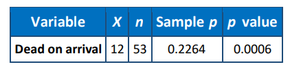
Which of the following conclusions can be reached?
I. The \(p\)-value of 0.0006 indicates that it is not very likely to get an observed value of 0.2264 if the null hypothesis is true.
II. The owner can be quite confident that this batch has significantly more “dead on arrival” batteries than the typical shipment.
III. The \(p\)-value of 0.0006 tells us that we cannot reject the null hypothesis and that the shipment has \(2 \%\) or less “dead on arrival” batteries.
A. I only
B. II only
C. III only
D. I and II only
E. II and III only
▶️Answer/Explanation
Explanation:
The correct answer is D. Statement I is true because the \(p\)-value is the probability of rejecting a true null hypothesis. As such, it is very unlikely to have gotten a test statistic value of 0.2264 if the null hypothesis is, in fact, true. Statement II is true because the \(p\)-value is so low that we reject the null hypothesis in favor of the alternative hypothesis that \(p>0.02\). So, the owner can be quite confident that this batch has significantly more “dead on arrival” batteries than the typical shipment. Statement III is false; this low of a \(p\)-value means that you \(d o\) reject the null hypothesis in favor of the alternative hypothesis.