Homogeneity Test
A chi-square homogeneity test determines whether two or more populations follow the same categorical distribution. The null hypothesis is that the distribution of the categorical variable across the populations is the same, whereas the alternative hypothesis is th at the distributions are not all the same. Note that this alternative does not preclude one or more of the values having the same proportions across populations, only that the overall distributions are not identical. The necessary conditions for this test are that the data come from a simple random sample, and that all expected counts be at least 5 .
Since the sample data come from two populations, it is represented in tabular form. The expected count for each cell in the table is given by \(E=\frac{(\text { row total }) \cdot(\text { column total })}{\text { table total }}\) The test statistic for the homogeneity test is \(\chi^2=\sum \frac{(O-E)^2}{E}\), just as with the goodness-of-fit test. However, the degrees of freedom is now equal to (number of rows – 1)(number of columns -1). As with the goodness-of-fit test, the \(p\)-value is given by the right tail of the appropriatechisquare distribution.
For example, the following table shows the number of men and women who responded to a question asking which of four factors they consider most important in the workplace. We will conduct a chi-square homogeneity test at the \(\alpha=0.1\) significance level.

The expected counts, calculated using the formula given, are as follows. For example, the first cell is calculated as \(\frac{30 \cdot 33}{90}=11\)

We can now calculate the test statistic. The first cell contributes \(\frac{(11-13)^2}{11} \approx 0.36\), the second cell contributes \(\frac{(5-5)^2}{5}=0\), and so on for the other six cells. The total for all of them is \(\chi^2 \approx 2.042\), and there are \((2-1)(4-1)=3\) degrees of freedom. The probability of obtaining a \(\chi^2\) of 2.042 or greater in this distribution is 0.5637 . Since \(p>\alpha\), we fail to reject the null hypothesis. There is not sufficient evidence to conclude that the distribution of this variable is different between men and women.
Sample Inference for Categorical Data: Chi-Square Questions
A survey was conducted to study people’s attitudes toward music containing explicit lyrics. A random sample of 1000 adults in the age categories \(18-25,26-35\), and \(36-45\) were selected to participate. They were classified according to age group and response to the question, “Do you think there is a link between listening to music containing explicit lyrics and bullying?”
The data are:
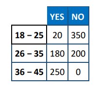
Which of the following statements is NOT correct?
A. The null hypothesis is that age category and opinion about bullying are independent.
B. The alternate hypothesis is that the proportion of people in various age groups who say YES is different from the proportion in various age groups who say NO.
C. A Type I error would be to conclude that opinions differed across age groups when, in fact, they do not.
D. A Type II error would be to conclude that opinions are the same across age groups when they are actually different.
E. The Chi-square test for independence cannot be performed because all cells must have nonzero entries in order to do so.
▶️Answer/Explanation
Explanation:
The correct answer is \(\mathrm{E}\). There is no such requirement to perform a Chi-square test. You might be mistaking observed frequencies for expected frequencies. Often, a minimum expected frequency of 5 is imposed to run this test, but this is not true of the observed frequencies. The other statements are all true.
Are all members of the kitchen staff equally prone to the same types of injuries? To investigate this question, a restaurant owner asks a consultant to classify accidents reported this month for all the restaurants she owns by type and the job performed in the kitchen. The results are tabulated below:
A Chi-square test for independence was performed and gave a test statistic of 11.24 . If we test at the significance level \(\alpha=0.05\), which of the following is true?
A. There appears to be no association between accident type and kitchen role.
B. Role seems to be independent of accident type.
C. Accident type does not seem to be independent of kitchen role.
D. There appears to be an \(11.24 \%\) correlation between accident type and kitchen role.
E. The proportion of sprains, burns, and cuts appear to be similar across all kitchen roles.
▶️Answer/Explanation
Explanation:
The correct answer is \(\mathrm{C}\). Note that \(\mathrm{df}=(3-1)(3-1)=4\). At the \(\alpha=0.05\) significance level, the cut-off for the critical region is 9.49 . Since the test statistic is larger than this value, we would reject the null hypothesis of independence of accident type and role in kitchen in favor of the existence of some association between them.
A random sample of 100 people was asked to state whether he or she graduated from college and to state his or her TV show preference (Reality TV, Sit-Coms, or Crime Drama). The results are provided below:
A Chi-square test is used to test the null hypothesis that college graduate status and TV show genre preference are independent. Which of the following statements is correct?
A. Accept \(\mathrm{H}_A\) at the 0.05 significance level
B. Reject \(\mathrm{H}_0\) at the 0.10 significance level
C. Reject \(\mathrm{H}_0\) at the 0.01 significance level
D. Reject \(\mathrm{H}_0\) at the 0.05 significance level
E. Accept \(\mathrm{H}_{\mathrm{A}}\) at the 0.01 significance level
▶️Answer/Explanation
Explanation:
The correct answer is B. Define the null and alternative hypotheses as follows:
\(\mathrm{H}_0\) : The probability of being in each cell is the product of the corresponding pair of marginal probabilities (that is, college graduate status and TV show genre preference are independent)
\(\mathrm{H}_{\mathrm{A}}\) : For at least one of the cells, the probability of belonging to that cell is not equal to the product of the corresponding pair of marginal probabilities (that is, college graduate status and TV show genre preference are not independent) Below are the observed and expected frequencies. In the cells, the observed O is the number outside the parentheses and the expected E is enclosed in parentheses.

Next, we compute \(\frac{(O-E)^2}{E}\) for each cell:

The test statistic is \(\chi^2=\grave{\circ} \frac{(O-E)^2}{E}=4.88\). Observe that \(\mathrm{df}=\) number of cells \(-1-\) number of parameters being estimated \(=6-1-3=2\).
The cut-off for the critical region with \(\alpha=0.01\) is 9.21 , with \(\alpha=0.05\) is 5.99 , and with \(\alpha=0.10\) is 4.61 .
Since the test statistic value is 4.88, we do not reject the null hypothesis at the significance levels \(\alpha=0.05\) or 0.01 , but we \(d o\) reject the null hypothesis at the \(\alpha=0.10\) level.