Home / 9709_m23_qp_62

Question 1

Topic – ALV: 5.3

Anita carried out a survey of 140 randomly selected students at her college. She found that 49 of these students watched a TV programme called Bunch.

(a) Calculate an approximate 98% confidence interval for the proportion, p, of students at Anita’s college who watch Bunch. 

Carlos says that the confidence interval found in (a) is not useful because it is too wide.

(b) Without calculation, explain briefly how Carlos can use the results of Anita’s survey to find a narrower confidence interval for p. 

▶️Answer/Explanation

Solution: –

(a) Calculate an approximate 98% confidence interval for \(p\).

Sample proportion \(\hat{p} = 49/140 \approx 0.35\), \(n = 140\).
For 98% confidence, \(z = 2.326\) (since \(\alpha/2 = 0.01\)).
Confidence interval:
\[
\hat{p} \pm z \cdot \sqrt{\frac{\hat{p}(1 – \hat{p})}{n}}
\]
\[
\sqrt{\frac{0.35 \cdot 0.65}{140}} = \sqrt{\frac{0.2275}{140}} = \sqrt{0.001625} \approx 0.0403
\]
\[
0.35 \pm 2.326 \cdot 0.0403 = 0.35 \pm 0.0937
\]
\[
0.2563 \leq p \leq 0.4437
\]
98% confidence interval: (0.256, 0.444) (to 3 decimal places).

(b) Explain briefly how Carlos can use the results to find a narrower confidence interval.

Carlos can increase the sample size \(n\). A larger \(n\) reduces the standard error \(\sqrt{\frac{\hat{p}(1 – \hat{p})}{n}}\), narrowing the confidence interval while maintaining the same confidence level (98%). This requires surveying more students to reduce variability in the estimate of \(p\).

————-Markscheme——————–

1(a)

$\hat{p}=0.35$

$0.35 \pm \sqrt{\frac{0.35(1-0.35)}{140}}$

z=2.326

Confidence interval = 0.256 to 0.444 (3 sf)

1(b)

Find a smaller percentage confidence interval/ lower level of confidence

Question 2

Topic – ALV: 5.2

The number of orders arriving at a shop during an 8-hour working day is modelled by the random variable $X$ with distribution $Po(25.2)$.

$(a)$ State two assumptions that are required for the Poisson model to be valid in this context. 

$(b)$

(i) Find the probability that the number of orders that arrive in a randomly chosen 3-hour period is between 3 and 5 inclusive. 

(ii) Find the probability that, in two randomly chosen 1-hour periods, exactly 1 order will arrive in one of the 1-hour periods, and at least 2 orders will arrive in the other 1-hour period. 

$(c)$ The shop can only deal with a maximum of 120 orders during any 36-hour period.

Use a suitable approximating distribution to find the probability that, in a randomly chosen 36-hour period, there will be too many orders for the shop to deal with.

▶️Answer/Explanation

Solution: –

(a) Assumptions for the Poisson Model

For a Poisson process to be a valid model, we assume:

  1. Independence: The number of orders arriving in one time period does not affect the number arriving in another time period.

  2. Constant Rate: Orders arrive at a constant average rate throughout the working hours, meaning the expected number of arrivals per unit time remains the same.


(b)

We are given that the number of orders arriving in an 8-hour day follows:

XPo(25.2)X \sim Po(25.2)

Since the Poisson process is time-scalable, the expected number of orders in a different time period is given by:

λnew=new time periodoriginal time period×λoriginal\lambda_{\text{new}} = \frac{\text{new time period}}{\text{original time period}} \times \lambda_{\text{original}}

(i) Probability for a 3-hour period

For a 3-hour period:

λ3h=38×25.2=9.45\lambda_{3h} = \frac{3}{8} \times 25.2 = 9.45

So the number of orders in a 3-hour period follows:

YPo(9.45)Y \sim Po(9.45)

We need to find:

P(3Y5)=P(Y=3)+P(Y=4)+P(Y=5)P(3 \leq Y \leq 5) = P(Y = 3) + P(Y = 4) + P(Y = 5)

Using the Poisson probability formula:

P(Y=k)=λkeλk!P(Y = k) = \frac{\lambda^k e^{-\lambda}}{k!}

for k=3,4,5k = 3, 4, 5, we have:

P(Y=3)=9.453e9.453!0.0111P(Y = 3) = \frac{9.45^3 e^{-9.45}}{3!} \approx 0.0111 P(Y=4)=9.454e9.454!0.0261P(Y = 4) = \frac{9.45^4 e^{-9.45}}{4!} \approx 0.0261 P(Y=5)=9.455e9.455!0.0494P(Y = 5) = \frac{9.45^5 e^{-9.45}}{5!} \approx 0.0494

Summing these:

P(3Y5)=0.0111+0.0261+0.0494=0.0866P(3 \leq Y \leq 5) = 0.0111 + 0.0261 + 0.0494 = 0.0866


(ii) Probability for two 1-hour periods

For a 1-hour period, we scale the mean:

λ1h=18×25.2=3.15\lambda_{1h} = \frac{1}{8} \times 25.2 = 3.15

So the number of orders in a 1-hour period follows:

ZPo(3.15)Z \sim Po(3.15)

We are given two independent 1-hour periods and want:

P(Exactly 1 order in one period and at least 2 orders in the other)P(\text{Exactly 1 order in one period and at least 2 orders in the other})

Let Z1Z_1 and Z2Z_2 be the orders in the two periods:

P(Z1=1)×P(Z22)+P(Z2=1)×P(Z12)P(Z_1 = 1) \times P(Z_2 \geq 2) + P(Z_2 = 1) \times P(Z_1 \geq 2)

Since the two periods are independent, we calculate:

P(Z=1)=3.151e3.151!0.1391P(Z = 1) = \frac{3.15^1 e^{-3.15}}{1!} \approx 0.1391 P(Z2)=1P(Z=0)P(Z=1)P(Z \geq 2) = 1 – P(Z = 0) – P(Z = 1) P(Z=0)=3.150e3.150!=e3.150.0429P(Z = 0) = \frac{3.15^0 e^{-3.15}}{0!} = e^{-3.15} \approx 0.0429 P(Z2)=1(0.0429+0.1391)=0.8180P(Z \geq 2) = 1 – (0.0429 + 0.1391) = 0.8180

Thus, the required probability is:

2×(0.1391×0.8180)=2×0.1139=0.22782 \times (0.1391 \times 0.8180) = 2 \times 0.1139 = 0.2278


(c) Approximating Distribution for a 36-hour Period

For a 36-hour period, we scale the mean:

λ36h=368×25.2=113.4\lambda_{36h} = \frac{36}{8} \times 25.2 = 113.4

Since λ=113.4\lambda = 113.4 is large, we approximate Po(113.4)Po(113.4) using a normal distribution:

N(μ=113.4,σ2=113.4)N(\mu = 113.4, \sigma^2 = 113.4)

where:

σ=113.410.65\sigma = \sqrt{113.4} \approx 10.65

We need to find:

P(X>120)P(X > 120)

Approximating using the normal distribution:

P(Z>120113.410.65)P\left( Z > \frac{120 – 113.4}{10.65} \right) =P(Z>6.610.65)= P\left( Z > \frac{6.6}{10.65} \right) =P(Z>0.62)= P(Z > 0.62)

Using standard normal tables:

P(Z>0.62)=1P(Z0.62)=10.7324=0.2676P(Z > 0.62) = 1 – P(Z \leq 0.62) = 1 – 0.7324 = 0.2676

Thus, the probability that there are too many orders for the shop to handle is 0.2676 (4 d.p.) or 26.8%.

————–Markscheme—————–

2(a)

Orders arrive at constant mean rate (must say mean or rate)
Orders arrive at random

Orders arrive independently
Orders arrive singly

2(b)(i)

$\lambda=\frac{3}{8}\times25.2[=9.45]$

$e^{-9.45}\left(\frac{9.45^{3}}{3!}+\frac{9.45^{4}}{4!}+\frac{9.45^{5}}{5!}\right)$ or $e^{-9.45}(140.65+332.29+628.03)$ or 0.01107 +
0.02615 + 0.04942

= 0.0866 (3 sf)

2(b)(ii)

$e^{-3.15}\times3.15$ or $(1-e^{-3.15})(1+3.15)$ or 0.135 or 0.822 (3 sf)

$e^{-3.15}\times3.15\times(1-e^{-3.15})(1+3.15)$

$\times 2$ or 0.111 × 2

0.222 (3 sf)

2(c)

N(113.4, 113.4)

$\frac{120.5-113.4}{\sqrt{113.4}}[=0.667]$

$1-\phi(their~’0.667′)$

= 0.252 (3 sf)

Question 3

Topic – ALV: 5.1

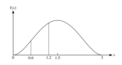
The diagram shows the graph of the probability density function, f, of a random variable X that takes values between $x=0$ and $x=3$ only. The graph is symmetrical about the line $x=1.5$.

(a) It is given that $P(X < 0.6) = a$ and $P(0.6 < X < 1.2) = b$.

Find $P(0.6 < X < 1.8)$ in terms of $a$ and $b$. 

(b) It is now given that the equation of the probability density function of X is

\[f(x)=\begin{cases}kx^{2}(3-x)^{2} & 0 < x < 3,\\ 0 & otherwise,\end{cases}\]

where k is a constant.

(i) Show that $k=\frac{10}{81}.$

(ii) Find Var(X).

▶️Answer/Explanation

Solution: –

The graph shows a symmetric probability density function (PDF) \(f(x)\) for a random variable \(X\), where \(0 \leq x \leq 3\), and the graph is symmetric about \(x = 1.5\). This suggests \(f(x)\) is likely a uniform or triangular distribution centered at \(x = 1.5\).

Understanding the Problem
– The total area under the PDF \(f(x)\) must equal 1 (since it’s a probability density function).
– Symmetry about \(x = 1.5\) means \(f(x) = f(3 – x)\) for \(0 \leq x \leq 3\).
– \(P(X < 0.6) = a\) is the area under \(f(x)\) from \(x = 0\) to \(x = 0.6\).
– \(P(0.6 < X < 1.2) = b\) is the area from \(x = 0.6\) to \(x = 1.2\).
– We need to find \(P(0.6 < X < 1.8)\) in terms of \(a\) and \(b\).

Step 1: Use Symmetry
Since the graph is symmetric about \(x = 1.5\), the area from \(x = 0\) to \(x = 1.5\) equals the area from \(x = 1.5\) to \(x = 3\), both being \(0.5\) (total probability = 1).

– \(P(X < 1.5) = 0.5\)
– \(P(1.5 < X < 3) = 0.5\)

Now, \(P(X < 0.6) = a\), so:
\[ P(0.6 < X < 1.5) = P(X < 1.5) – P(X < 0.6) = 0.5 – a \]

Due to symmetry about \(x = 1.5\), the area from \(x = 1.5\) to \(x = 2.4\) (which is \(3 – 0.6\)) equals the area from \(x = 0.6\) to \(x = 1.5\):
\[ P(1.5 < X < 2.4) = 0.5 – a \]

Step 2: Relate \(b\) to the Given Intervals
\(P(0.6 < X < 1.2) = b\). Notice:
– The interval \(0.6 < X < 1.2\) is half of the symmetric interval around \(x = 1.5\), from \(1.5 – 0.6 = 0.9\) to \(1.5 + 0.6 = 2.1\), but we’re given \(0.6\) to \(1.2\).

Using symmetry again, the area from \(1.2\) to \(1.5\) should equal the area from \(1.5\) to \(1.8\) (since \(1.8 = 3 – 1.2\)):
\[ P(1.2 < X < 1.5) = P(1.5 < X < 1.8) \]

Now:
\[ P(0.6 < X < 1.5) = P(0.6 < X < 1.2) + P(1.2 < X < 1.5) = b + P(1.2 < X < 1.5) \]

But \(P(0.6 < X < 1.5) = 0.5 – a\), so:
\[ 0.5 – a = b + P(1.2 < X < 1.5) \]
\[ P(1.2 < X < 1.5) = 0.5 – a – b \]

By symmetry:
\[ P(1.5 < X < 1.8) = 0.5 – a – b \]

### Step 3: Find \(P(0.6 < X < 1.8)\)
\[ P(0.6 < X < 1.8) = P(0.6 < X < 1.2) + P(1.2 < X < 1.5) + P(1.5 < X < 1.8) \]
\[ = b + (0.5 – a – b) + (0.5 – a – b) \]
\[ = b + 0.5 – a – b + 0.5 – a – b \]
\[ = 1 – 2a – b \]

Final Answer
\[ P(0.6 < X < 1.8) = 1 – 2a – b \]

(b)(i) Show that \(k = \frac{10}{81}\)

The function \(f(x)\) is the probability density function (PDF) of \(X\), where \(0 < x < 3\), and \(f(x) = 0\) otherwise. For \(f(x)\) to be a valid PDF, the total area under the curve must equal 1:

\[ \int_{-\infty}^{\infty} f(x) \, dx = 1 \]

Since \(f(x) = 0\) outside \(0 < x < 3\), we integrate:

\[ \int_0^3 kx^2(3 – x)^2 \, dx = 1 \]

First, expand \((3 – x)^2\):

\[ (3 – x)^2 = 9 – 6x + x^2 \]

\[ x^2(3 – x)^2 = x^2(9 – 6x + x^2) = 9x^2 – 6x^3 + x^4 \]

Now integrate:

\[ \int_0^3 (9x^2 – 6x^3 + x^4) \, dx = k \cdot 1 \]

Compute the integral:

\[ \int_0^3 9x^2 \, dx = 9 \left[ \frac{x^3}{3} \right]_0^3 = 9 \cdot \frac{3^3}{3} = 9 \cdot 9 = 81 \]
\[ \int_0^3 -6x^3 \, dx = -6 \left[ \frac{x^4}{4} \right]_0^3 = -6 \cdot \frac{3^4}{4} = -6 \cdot \frac{81}{4} = -\frac{486}{4} = -121.5 \]
\[ \int_0^3 x^4 \, dx = \left[ \frac{x^5}{5} \right]_0^3 = \frac{3^5}{5} = \frac{243}{5} = 48.6 \]

Sum them:

\[ 81 – 121.5 + 48.6 = 81 – 121.5 + 48.6 = 8.1 \]

So:

\[ k \cdot 8.1 = 1 \]
\[ k = \frac{1}{8.1} = \frac{1}{\frac{81}{10}} = \frac{10}{81} \]

Thus, \(k = \frac{10}{81}\).

(b)(ii) Find \(\text{Var}(X)\)

Variance \(\text{Var}(X) = E(X^2) – [E(X)]^2\).

Step 1: Find \(E(X)\)
\[ E(X) = \int_0^3 x \cdot f(x) \, dx = \int_0^3 x \cdot \frac{10}{81} x^2 (3 – x)^2 \, dx = \frac{10}{81} \int_0^3 x^3 (3 – x)^2 \, dx \]

Use \((3 – x)^2 = 9 – 6x + x^2\):

\[ x^3 (3 – x)^2 = x^3 (9 – 6x + x^2) = 9x^3 – 6x^4 + x^5 \]

Integrate:

\[ \int_0^3 9x^3 \, dx = 9 \left[ \frac{x^4}{4} \right]_0^3 = 9 \cdot \frac{3^4}{4} = 9 \cdot \frac{81}{4} = \frac{729}{4} = 182.25 \]
\[ \int_0^3 -6x^4 \, dx = -6 \left[ \frac{x^5}{5} \right]_0^3 = -6 \cdot \frac{3^5}{5} = -6 \cdot \frac{243}{5} = -\frac{1458}{5} = -291.6 \]
\[ \int_0^3 x^5 \, dx = \left[ \frac{x^6}{6} \right]_0^3 = \frac{3^6}{6} = \frac{729}{6} = 121.5 \]

Sum:

\[ 182.25 – 291.6 + 121.5 = 182.25 – 291.6 + 121.5 = 12.15 \]

\[ E(X) = \frac{10}{81} \cdot 12.15 = \frac{10}{81} \cdot \frac{1215}{100} = \frac{10 \cdot 1215}{81 \cdot 100} = \frac{12150}{8100} = \frac{1215}{810} = \frac{405}{270} = \frac{3}{2} \]

Step 2: Find \(E(X^2)\)
\[ E(X^2) = \int_0^3 x^2 \cdot f(x) \, dx = \int_0^3 x^2 \cdot \frac{10}{81} x^2 (3 – x)^2 \, dx = \frac{10}{81} \int_0^3 x^4 (3 – x)^2 \, dx \]

\[ x^4 (3 – x)^2 = x^4 (9 – 6x + x^2) = 9x^4 – 6x^5 + x^6 \]

Integrate:

\[ \int_0^3 9x^4 \, dx = 9 \left[ \frac{x^5}{5} \right]_0^3 = 9 \cdot \frac{3^5}{5} = 9 \cdot \frac{243}{5} = \frac{2187}{5} = 437.4 \]
\[ \int_0^3 -6x^5 \, dx = -6 \left[ \frac{x^6}{6} \right]_0^3 = -6 \cdot \frac{3^6}{6} = -6 \cdot \frac{729}{6} = -729 \]
\[ \int_0^3 x^6 \, dx = \left[ \frac{x^7}{7} \right]_0^3 = \frac{3^7}{7} = \frac{2187}{7} \approx 312.4286 \]

Sum:

\[ 437.4 – 729 + 312.4286 = 437.4 – 729 + 312.4286 = 20.8286 \]

\[ E(X^2) = \frac{10}{81} \cdot 20.8286 = \frac{10}{81} \cdot \frac{1458}{70} = \frac{10 \cdot 1458}{81 \cdot 70} = \frac{14580}{5670} = \frac{729}{283.5} \]

Simplify:

\[ \frac{14580}{5670} = \frac{1458}{567} = \frac{486}{189} = \frac{162}{63} = \frac{54}{21} = \frac{18}{7} \]

Step 3: Compute Variance
\[ \text{Var}(X) = E(X^2) – [E(X)]^2 = \frac{18}{7} – \left(\frac{3}{2}\right)^2 \]
\[ \left(\frac{3}{2}\right)^2 = \frac{9}{4} \]
\[ \frac{18}{7} – \frac{9}{4} = \frac{18 \cdot 4 – 9 \cdot 7}{7 \cdot 4} = \frac{72 – 63}{28} = \frac{9}{28} \]

Final Answers
(i) \(k = \frac{10}{81}\)
(ii) \(\text{Var}(X) = \frac{9}{28}\)

———————-Markscheme——————–

(a)

$1-2(a+b)$ or $1-2a$ or $0.5-a-b$ or $1-(a+b)$ or $a+a+b$

$P(0.6\le X\le1.8)=1-2a-b$

(b)(i)

$k\int_{0}^{3}(9x^{2}-6x^{3}+x^{4})dx=1$

$k[\frac{9x^{3}}{3}-\frac{6x^{4}}{4}+\frac{x^{5}}{5}]_{0}^{3}=1$

$k\times\frac{81}{10}=1, k=\frac{10}{81}$

(b)(ii)

$\frac{10}{81}\int_{0}^{3}(9x^{4}-6x^{5}+x^{6})dx$

$\frac{10}{81}[\frac{9x^{5}}{5}-\frac{6x^{6}}{6}+\frac{x^{7}}{7}]_{0}^{3}=\left[\frac{18}{7}~or~2.57…\right]$

$\frac{18}{7}-1.5^{2}$

$=\frac{9}{28}~or~0.321$

Question 4

Topic – ALV: 5.2

The number of accidents per 3-month period on a certain road has the distribution $Po(\lambda)$. In the past the value of $\lambda$ has been 5.7. Following some changes to the road, the council carries out a hypothesis test to determine whether the value of $\lambda$ has decreased. If there are fewer than 3 accidents in a randomly chosen 3-month period, the council will conclude that the value of $\lambda$ has decreased.

(a) Find the probability of a Type I error.

(b) Find the probability of a Type II error if the mean number of accidents per 3-month period is now actually 0.9. 

▶️Answer/Explanation

Solution: –

The number of accidents per 3-month period follows a Poisson distribution \(Po(\lambda)\), where \(\lambda\) was previously 5.7. The council tests whether \(\lambda\) has decreased, using the hypothesis test:
– Null hypothesis \(H_0\): \(\lambda = 5.7\) (no decrease).
– Alternative hypothesis \(H_1\): \(\lambda < 5.7\) (decrease).
– Test rule: Reject \(H_0\) if there are fewer than 3 accidents (i.e., 0, 1, or 2 accidents) in a randomly chosen 3-month period.

(a) Find the probability of a Type I error

A Type I error occurs when \(H_0\) is true (\(\lambda = 5.7\)) but is rejected (i.e., the number of accidents is 0, 1, or 2).

For \(Po(5.7)\), calculate \(P(X < 3) = P(X = 0) + P(X = 1) + P(X = 2)\), where \(X \sim Po(5.7)\):

\[ P(X = k) = \frac{\lambda^k e^{-\lambda}}{k!} \]

– \(P(X = 0) = \frac{5.7^0 e^{-5.7}}{0!} = e^{-5.7}\)
– \(P(X = 1) = \frac{5.7^1 e^{-5.7}}{1!} = 5.7 e^{-5.7}\)
– \(P(X = 2) = \frac{5.7^2 e^{-5.7}}{2!} = \frac{5.7^2 e^{-5.7}}{2}\)

First, \(e^{-5.7} \approx 0.003311\):

\[ 5.7^2 = 32.49 \]
\[ P(X = 2) = \frac{32.49 \cdot 0.003311}{2} \approx \frac{0.10755}{2} = 0.053775 \]

Now sum:

\[ P(X = 0) \approx 0.003311 \]
\[ P(X = 1) \approx 5.7 \cdot 0.003311 \approx 0.018877 \]
\[ P(X = 2) \approx 0.053775 \]

\[ P(X < 3) \approx 0.003311 + 0.018877 + 0.053775 = 0.075963 \]

So, the probability of a Type I error is approximately:

\[ \text{Type I error} \approx 0.076 \]

(b) Find the probability of a Type II error if \(\lambda = 0.9\)

A Type II error occurs when \(H_1\) is true (\(\lambda = 0.9\)) but \(H_0\) is not rejected (i.e., the number of accidents is 3 or more, \(X \geq 3\)).

For \(X \sim Po(0.9)\), calculate \(P(X \geq 3) = 1 – P(X < 3) = 1 – [P(X = 0) + P(X = 1) + P(X = 2)]\):

– \(P(X = 0) = e^{-0.9} \approx e^{-0.9} \approx 0.40657\)
– \(P(X = 1) = 0.9 e^{-0.9} \approx 0.9 \cdot 0.40657 = 0.365913\)
– \(P(X = 2) = \frac{0.9^2 e^{-0.9}}{2} = \frac{0.81 \cdot 0.40657}{2} \approx \frac{0.32932}{2} = 0.16466\)

\[ P(X < 3) \approx 0.40657 + 0.365913 + 0.16466 = 0.937143 \]

\[ P(X \geq 3) = 1 – 0.937143 = 0.062857 \]

So, the probability of a Type II error is approximately:

\[ \text{Type II error} \approx 0.063 \]

Final Answers
(a) Probability of Type I error = 0.076
(b) Probability of Type II error (\(\lambda = 0.9\)) = 0.063

——————Markscheme————–

(a)

$e^{-5.7}(1+5.7+\frac{5.7^{2}}{2!})$ or $e^{-5.7}(1+5.7+16.245)$ or 0.003346 + 0.01907 + 0.05436

= 0.0768 (3 sf)

(b)

$e^{-0.9}(1+0.9+\frac{0.9^{2}}{2!})$

$=1-e^{-0.9}(1+0.9+\frac{0.9^{2}}{2!})=1-e^{-0.9}(1+0.9+0.405)=1-(0.4066+3659+0.1647)$

= 0.0629 (3 sf)


Question 5

Topic – ALV: 5.2

The masses, in grams, of large and small packets of Max wheat cereal have the independent distributions

$N(410.0, 3.6^2)$ and $N(206.0, 3.7^2)$ respectively.

(a) Find the probability that a randomly chosen large packet has a mass that is more than double the mass of a randomly chosen small packet.

The packets are placed in boxes. The boxes are identical in appearance. 60% of the boxes contain exactly 10 randomly chosen large packets. 40% of the boxes contain exactly 20 randomly chosen small packets.

(b) Find the probability that a randomly chosen box contains packets with a total mass of more than 4080 grams.

▶️Answer/Explanation

Solution: –

(a) Probability that a large packet has more than double the mass of a small packet

Let:

  • XN(410.0,3.62)X \sim N(410.0, 3.6^2) be the mass of a large packet.
  • YN(206.0,3.72)Y \sim N(206.0, 3.7^2) be the mass of a small packet.

We need to find:

P(X>2Y)P(X > 2Y)

Define D=X2YD = X – 2Y. Then,

D=X2YN(μD,σD2)D = X – 2Y \sim N\left( \mu_D, \sigma_D^2 \right)

where:

μD=E(X)2E(Y)=410.02(206.0)=2.0\mu_D = E(X) – 2E(Y) = 410.0 – 2(206.0) = -2.0 σD2=Var(X)+4Var(Y)=3.62+4(3.72)\sigma_D^2 = \text{Var}(X) + 4\text{Var}(Y) = 3.6^2 + 4(3.7^2) =12.96+4(13.69)=12.96+54.76=67.72= 12.96 + 4(13.69) = 12.96 + 54.76 = 67.72 σD=67.728.23\sigma_D = \sqrt{67.72} \approx 8.23

We now find:

P(D>0)=P(Z>0(2.0)8.23)=P(Z>2.08.23)P(D > 0) = P\left( Z > \frac{0 – (-2.0)}{8.23} \right) = P\left( Z > \frac{2.0}{8.23} \right) =P(Z>0.243)= P(Z > 0.243)

From normal tables:

P(Z>0.243)=1P(Z0.243)=10.596P(Z > 0.243) = 1 – P(Z \leq 0.243) = 1 – 0.596 =0.404= 0.404

Final answer:

P(X>2Y)=0.404 (3 d.p.)P(X > 2Y) = 0.404 \text{ (3 d.p.)}


(b) Probability that a randomly chosen box contains a total mass of more than 4080 g

The box can contain:

  1. 10 large packets (60% probability) → Total mass:

    SL=10XN(10(410.0),10(3.62))S_L = 10X \sim N(10(410.0), 10(3.6^2)) =N(4100,129.6)= N(4100, 129.6) σL=129.611.39\sigma_L = \sqrt{129.6} \approx 11.39
  2. 20 small packets (40% probability) → Total mass:

    SS=20YN(20(206.0),20(3.72))S_S = 20Y \sim N(20(206.0), 20(3.7^2)) =N(4120,273.8)= N(4120, 273.8) σS=273.816.55\sigma_S = \sqrt{273.8} \approx 16.55

We need to find:

P(S>4080)=P(SL>4080)PL+P(SS>4080)PSP(S > 4080) = P(S_L > 4080) P_L + P(S_S > 4080) P_S

where:

P(SL>4080)=P(Z>4080410011.39)=P(Z>2011.39)=P(Z>1.755)P(S_L > 4080) = P\left( Z > \frac{4080 – 4100}{11.39} \right) = P\left( Z > \frac{-20}{11.39} \right) = P(Z > -1.755)

Using normal tables:

P(Z>1.755)=1P(Z1.755)=10.0395=0.9605P(Z > -1.755) = 1 – P(Z \leq -1.755) = 1 – 0.0395 = 0.9605

Similarly,

P(SS>4080)=P(Z>4080412016.55)=P(Z>4016.55)=P(Z>2.417)P(S_S > 4080) = P\left( Z > \frac{4080 – 4120}{16.55} \right) = P\left( Z > \frac{-40}{16.55} \right) = P(Z > -2.417) P(Z>2.417)=1P(Z2.417)=10.0078=0.9922P(Z > -2.417) = 1 – P(Z \leq -2.417) = 1 – 0.0078 = 0.9922

Now, using:

P(S>4080)=(0.9605×0.6)+(0.9922×0.4)P(S > 4080) = (0.9605 \times 0.6) + (0.9922 \times 0.4) =0.5763+0.3969=0.9732= 0.5763 + 0.3969 = 0.9732

Final answer:

P(S>4080)=0.973 (3 d.p.)P(S > 4080) = 0.973 \text{ (3 d.p.)}

————Markscheme———-

(a)

$D=L-2S$

$E(D)=410-2(206)=-2$

$Var(D)=3.6^{2}+4\times3.7^{2}$ $[=67.72]$

$\frac{0-(-2)}{\sqrt{67.72^{\circ}}}$

$[=0.243]$

$1-\Phi(their^{\circ}0.243^{\circ})$

$= 0.404 (3 sf)$

(b)

$T_{L}\sim N(4100,10\times3.6^{2})$

$T_{S}\sim N(4120,20\times3.7^{2})$

$\frac{4080-4100}{\sqrt{129.6^{\prime}}}(=-1.757)$

$\frac{4080-4120}{\sqrt{273.8^{7}}}(=-2.417)$

$1-\Phi(-1.757^{\prime})=\Phi(1.757)$

$1-\Phi(-2.417^{\prime})=\Phi(2.417)$

= 0.9605~or~0.961

= 0.9921 or 0.9922 or 0.992

$= 0.973 (3~sf)$


Question 6

Topic – ALV: 5.1

Last year, the mean time taken by students at a school to complete a certain test was 25 minutes. Akash believes that the mean time taken by this year’s students was less than 25 minutes. In order to test this belief, he takes a large random sample of this year’s students and he notes the time taken by each student. He carries out a test, at the 2.5% significance level, for the population mean time, μ minutes. Akash uses the null hypothesis H₀: μ = 25.

(a) Give a reason why Akash should use a one-tailed test. 

Akash finds that the value of the test statistic is $z = -2.02$.

(b) Explain what conclusion he should draw. 

In a different one-tailed hypothesis test the z-value was found to be 2.14.

(c) Given that this value would lead to a rejection of the null hypothesis at the α% significance level, find the set of possible values of α. 

The population mean time taken by students at another school to complete a test last year was m minutes. Sorin carries out a one-tailed test to determine whether the population mean this year is less than m, using a random sample of 100 students. He assumes that the population standard deviation of the times is 3.9 minutes. The sample mean is 24.8 minutes, and this result just leads to the rejection of the null hypothesis at the 5% significance level.

(d) Find the value of m. 

▶️Answer/Explanation

Solution: –

(a) Reason for a One-Tailed Test

Akash believes that the mean time taken this year is less than last year’s mean of 25 minutes. This suggests a directional hypothesis:

H1:μ<25H_1: \mu < 25

Since we are only testing whether the mean has decreased (and not whether it has changed in any direction), a one-tailed test is appropriate.


(b) Conclusion for z=2.02z = -2.02

For a one-tailed test at the 2.5% significance level, we check the critical value from the standard normal distribution.

From normal tables:

P(Z<1.960)=0.025P(Z < -1.960) = 0.025

Since the test is one-tailed, we reject H0H_0 if:

z<1.960z < -1.960

Given that Akash’s test statistic is:

z=2.02z = -2.02

which is less than -1.960, we reject the null hypothesis.

Conclusion: There is sufficient evidence at the 2.5% significance level to conclude that the mean test time this year is less than 25 minutes.


(c) Finding the Set of Possible Values of α\alpha

Given that z=2.14z = 2.14 leads to rejection of H0H_0, we need to find the largest possible α\alpha level for which the null hypothesis is rejected.

In a one-tailed test, we reject H0H_0 if:

P(Z>2.14)<αP(Z > 2.14) < \alpha

From normal tables:

P(Z>2.14)=1P(Z2.14)=10.9838=0.0162P(Z > 2.14) = 1 – P(Z \leq 2.14) = 1 – 0.9838 = 0.0162

Since this pp-value corresponds to the largest α\alpha that would still result in rejection, we conclude:

α>0.0162\alpha > 0.0162

Answer: α>1.62%\alpha > 1.62\%. That is, the test must be at a significance level greater than 1.62%.


(d) Finding mm

Sorin carries out a one-tailed test with:

  • Sample size: n=100n = 100
  • Sample mean: xˉ=24.8\bar{x} = 24.8
  • Population standard deviation: σ=3.9\sigma = 3.9
  • Significance level: 5%
  • The test just leads to rejection of H0H_0, meaning the test statistic is at the critical value.

For a one-tailed test at 5%, the critical value is:

z=1.645z = -1.645

Using the test statistic formula:

z=xˉmσ/nz = \frac{\bar{x} – m}{\sigma / \sqrt{n}}

Substituting known values:

1.645=24.8m3.9/100-1.645 = \frac{24.8 – m}{3.9 / \sqrt{100}} 1.645=24.8m3.9/10-1.645 = \frac{24.8 – m}{3.9 / 10} 1.645=24.8m0.39-1.645 = \frac{24.8 – m}{0.39}

Solving for mm:

24.8m=1.645×0.3924.8 – m = -1.645 \times 0.39 24.8m=0.641624.8 – m = -0.6416 m=24.8+0.6416m = 24.8 + 0.6416 m=25.44m = 25.44

Final Answer: m=25.44m = 25.44 (2 d.p.)

———–Markscheme—————

(a)

He is expecting a decrease (in μ)

(b)

$-2.02<-1.96$

$(Reject H_{0})$

There is evidence to suggest that this year’s (mean) time is less than 25

(c)

$1-\Phi(2.14)[=0.0162]$

$1.62$

$\alpha \ge 1.62$ (3 sf)

(d)

$\frac{24.8-m}{3.9+10}$

$\frac{24.8-m}{3.9+10}=-1.645$

$m=25.4$ (3 sf)

Scroll to Top