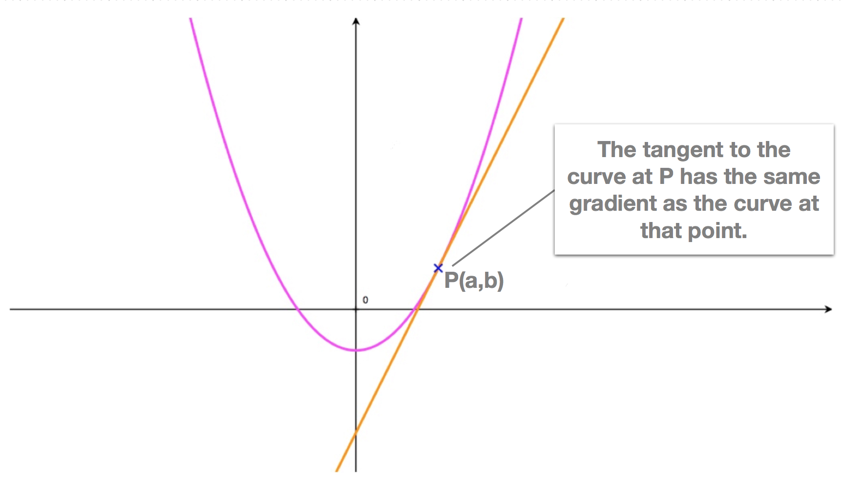
Gradient of a Curve at a Point
The gradient (slope) of a curve at a point is the slope of the tangent to the curve at that point. It represents the rate of change of \(y\) with respect to \(x\) at a single point.
Gradient as the Limit of Chord Gradients
Consider a curve \(y = f(x)\) and a point \(P(x, f(x))\) on it. Take another point \(Q(x+h, f(x+h))\) close to \(P\). The slope of the chord joining \(P\) and \(Q\) is: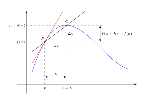
\(\text{Gradient of chord} = \dfrac{f(x+h) – f(x)}{h}\)
As \(Q\) moves closer to \(P\) (\(h \to 0\)), the chord approaches the tangent at \(P\). Therefore, the gradient of the tangent is:
\(\text{Gradient of tangent at } P = \lim_{h \to 0} \dfrac{f(x+h) – f(x)}{h}\)
This is also called the first derivative of \(f\) at \(x = a\):
\(f'(a) = \lim_{h \to 0} \dfrac{f(a+h) – f(a)}{h}\)
Notation for First and Second Derivatives
- First derivative (gradient of the curve): \(f'(x)\) or \(\dfrac{dy}{dx}\)
- Second derivative (rate of change of gradient / concavity of the curve): \(f”(x)\) or \(\dfrac{d^2y}{dx^2}\)
Interpretation: 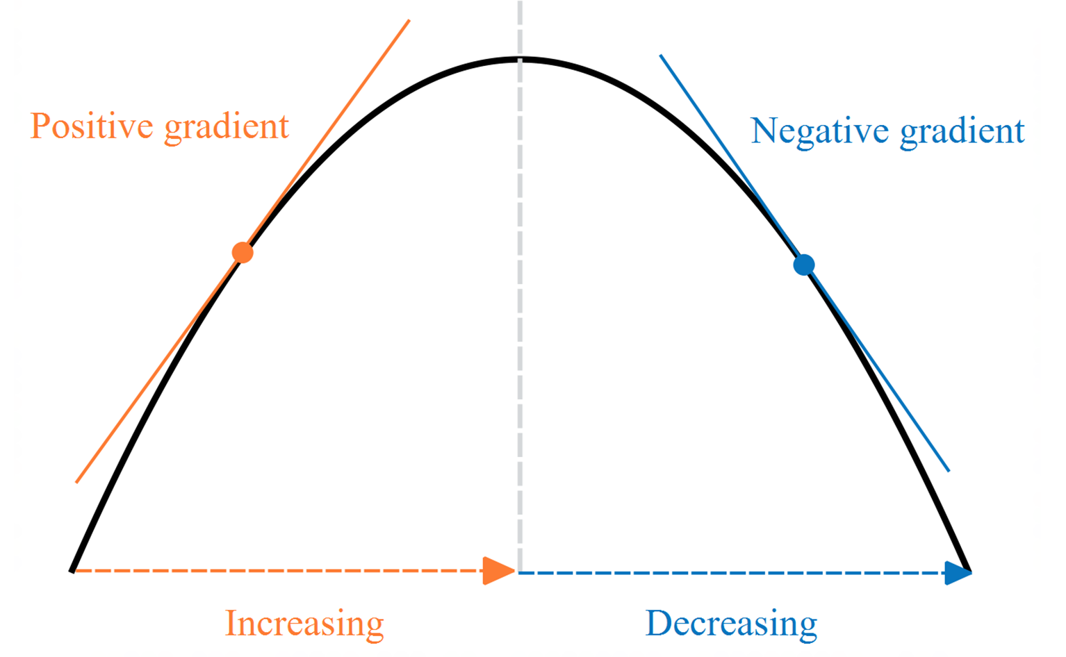
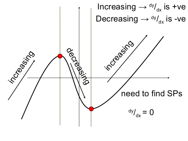
- \(f'(x) > 0\): curve is increasing
- \(f'(x) < 0\): curve is decreasing
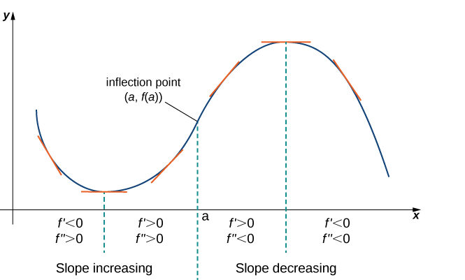
- \(f”(x) > 0\): curve is concave up (gradient increasing)
- \(f”(x) < 0\): curve is concave down (gradient decreasing)
Key Points:
- The gradient at a point is the limit of the gradients of nearby chords.
- First derivative gives the slope of the tangent; second derivative gives concavity.
- Notation: \(f'(x)\) or \(\dfrac{dy}{dx}\) for first derivative; \(f”(x)\) or \(\dfrac{d^2y}{dx^2}\) for second derivative.
- Use limit definition for conceptual understanding; derivative formulas for practical calculations.
Example:
Find the gradient of the curve \(y = \dfrac{1}{x}\) at \(x = 1\) using the limit definition.
▶️ Answer/Explanation
Step 1: Gradient of a chord
\(\dfrac{f(1+h) – f(1)}{h} = \dfrac{\dfrac{1}{1+h} – 1}{h} = \dfrac{\dfrac{1 – (1+h)}{1+h}}{h} = \dfrac{-h}{h(1+h)} = \dfrac{-1}{1+h}\)
Step 2: Take the limit as \(h \to 0\)
\(\lim_{h \to 0} \dfrac{-1}{1+h} = -1\)
Step 3: Derivative notation
\(f'(x) = -\dfrac{1}{x^2} \implies f'(1) = -1\)
Final Answer: Gradient at \(x = 1\) is -1
Example
Find the first and second derivatives of \(y = x^3 – 3x^2 + 2x\), and evaluate them at \(x = 1\).
▶️ Answer/Explanation
Step 1: First derivative
\(y’ = f'(x) = 3x^2 – 6x + 2\)
At \(x = 1\), \(f'(1) = 3 – 6 + 2 = -1\)
Step 2: Second derivative
\(y” = f”(x) = 6x – 6\)
At \(x = 1\), \(f”(1) = 6 – 6 = 0\)
Final Answer: \(f'(1) = -1\), \(f”(1) = 0\)
Example
Find the gradient of \(y = \sqrt{x+1}\) at \(x = 3\).
▶️ Answer/Explanation
Step 1: Use derivative formula for square root
\(y’ = \dfrac{1}{2\sqrt{x+1}}\)
Step 2: Evaluate at \(x = 3\)
\(y'(3) = \dfrac{1}{2\sqrt{3+1}} = \dfrac{1}{2\cdot 2} = \dfrac{1}{4}\)
Final Answer: Gradient at \(x = 3\) is \(\dfrac{1}{4}\)
Example:
Find the gradient of the tangent to the curve \(y = x^3\) at \(x = 2\) using the limit of the gradient of the chord joining points \((2, f(2))\) and \((2+h, f(2+h))\).
▶️ Answer/Explanation
Step 1: Gradient of the chord
\(\text{Gradient of chord} = \dfrac{f(2+h) – f(2)}{h} = \dfrac{(2+h)^3 – 2^3}{h} = \dfrac{8 + 12h + 6h^2 + h^3 – 8}{h} = \dfrac{12h + 6h^2 + h^3}{h} = 12 + 6h + h^2\)
Step 2: Take the limit as \(h \to 0\)
\(\lim_{h \to 0} (12 + 6h + h^2) = 12\)
Step 3: Using derivative notation
\(f'(x) = 3x^2 \implies f'(2) = 3(2)^2 = 12\)
Final Answer: Gradient of the tangent at \(x = 2\) is 12
Derivatives of Functions
We can now move from the definition of the derivative to rules for differentiation. These allow us to find derivatives of more complicated functions efficiently.
Power Rule (for any rational \(n\))
If \(y = x^n\), where \(n\) is any rational number, then:
\(\dfrac{dy}{dx} = n x^{n-1}\)
Examples: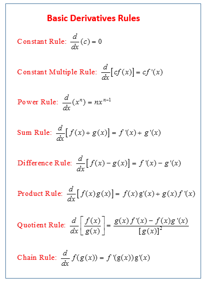
- \(\dfrac{d}{dx}(x^5) = 5x^4\)
- \(\dfrac{d}{dx}(x^{\tfrac{1}{2}}) = \dfrac{1}{2} x^{-\tfrac{1}{2}}\)
- \(\dfrac{d}{dx}(x^{-3}) = -3x^{-4}\)
Constant Multiple Rule
If \(y = k f(x)\), where \(k\) is a constant, then:
\(\dfrac{dy}{dx} = k \dfrac{d}{dx}(f(x))\)
Sum and Difference Rule
If \(y = f(x) + g(x)\) or \(y = f(x) – g(x)\), then:
\(\dfrac{dy}{dx} = f'(x) + g'(x)\) or \(\dfrac{dy}{dx} = f'(x) – g'(x)\)
Chain Rule (for composite functions)
If \(y = f(g(x))\), then:
\(\dfrac{dy}{dx} = f'(g(x)) \cdot g'(x)\)
Another way to write:
\(\dfrac{dy}{dx} = \dfrac{dy}{du} \cdot \dfrac{du}{dx}\), where \(u = g(x)\).
Example:
Differentiate \(y = 7x^{\tfrac{3}{2}}\).
▶️ Answer/Explanation
\(\dfrac{dy}{dx} = 7 \cdot \dfrac{3}{2} x^{\tfrac{1}{2}} = \dfrac{21}{2} \sqrt{x}\)
Final Answer: \(\dfrac{dy}{dx} = \dfrac{21}{2}\sqrt{x}\)
Example:
Differentiate \(y = 4x^3 – \dfrac{5}{x^2}\).
▶️ Answer/Explanation
\(\dfrac{dy}{dx} = 12x^2 – 5(-2)x^{-3} = 12x^2 + \dfrac{10}{x^3}\)
Final Answer: \(\dfrac{dy}{dx} = 12x^2 + \dfrac{10}{x^3}\)
Example:
Differentiate \(y = (3x^2 + 1)^5\).
▶️ Answer/Explanation
Let \(u = 3x^2 + 1 \implies y = u^5\).
\(\dfrac{dy}{du} = 5u^4, \quad \dfrac{du}{dx} = 6x\).
\(\dfrac{dy}{dx} = 5(3x^2+1)^4 \cdot 6x = 30x(3x^2+1)^4\).
Final Answer: \(\dfrac{dy}{dx} = 30x(3x^2+1)^4\)
Gradients, Tangents, and Normals
The derivative of a function \(y = f(x)\) gives the gradient of the curve at any point.
- Gradient of the curve at \(x = a\): \(f'(a)\).
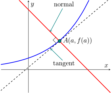
- Equation of the tangent: A tangent touches the curve at exactly one point and has slope \(f'(a)\). Equation: \(y – y_1 = f'(a)(x – a)\).
- Equation of the normal: A normal is perpendicular to the tangent. Its slope is the negative reciprocal of the tangent slope. Equation: \(y – y_1 = -\dfrac{1}{f'(a)}(x – a)\).
This is used in curve sketching and in geometry problems involving perpendicular lines.
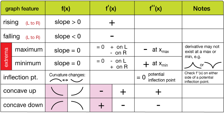
Increasing and Decreasing Functions
The derivative also tells us where the function is rising or falling:
- If \(f'(x) > 0\), the curve is increasing (gradient is positive).
- If \(f'(x) < 0\), the curve is decreasing (gradient is negative).
- If \(f'(x) = 0\), the curve has a stationary point. At these points:
- If \(f”(x) > 0\), the point is a local minimum (curve bends upwards).
- If \(f”(x) < 0\), the point is a local maximum (curve bends downwards).
- If \(f”(x) = 0\), further investigation is needed (could be a point of inflection).
This analysis is important in optimization problems and curve sketching.
Rates of Change
Many problems involve quantities changing with respect to time. If two variables are related, say \(y = f(x)\), and \(x\) depends on time \(t\), then we apply the chain rule: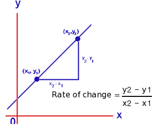
\(\dfrac{dy}{dt} = \dfrac{dy}{dx} \cdot \dfrac{dx}{dt}\)
This means the rate of change of \(y\) with respect to time depends on both the derivative \(\dfrac{dy}{dx}\) and the rate of change of \(x\) with respect to time.
Applications include:
- Finding how fast an area changes as a radius increases.
- Finding how fast the volume of a balloon changes as it is inflated.
- Related rates problems (e.g. a ladder sliding down a wall).
Example:
Find the equations of the tangent and normal to the curve \(y = x^2 + 3x\) at \(x = 1\).
▶️ Answer/Explanation
\(f'(x) = 2x + 3\). At \(x=1\), gradient = \(2(1) + 3 = 5\).
Point: \((1, 1^2 + 3(1)) = (1, 4)\).
Tangent: \(y – 4 = 5(x – 1)\).
Normal: Gradient = \(-\dfrac{1}{5}\). Equation: \(y – 4 = -\dfrac{1}{5}(x – 1)\).
Final Answers:
Tangent: \(y = 5x – 1\)
Normal: \(y = -\dfrac{1}{5}x + \dfrac{21}{5}\)
Example :
Determine the intervals where \(f(x) = x^3 – 3x^2\) is increasing or decreasing.
▶️ Answer/Explanation
\(f'(x) = 3x^2 – 6x = 3x(x – 2)\).
Critical points: \(x = 0, 2\).
- For \(x < 0\), pick \(x = -1\): \(f'(-1) = 3(-1)(-3) = 9 > 0\) → Increasing.
- For \(0 < x < 2\), pick \(x = 1\): \(f'(1) = 3(1)(-1) = -3 < 0\) → Decreasing.
- For \(x > 2\), pick \(x = 3\): \(f'(3) = 3(3)(1) = 9 > 0\) → Increasing.
Final Answer: Increasing on \((-\infty, 0) \cup (2, \infty)\), Decreasing on \((0, 2)\).
Example:
The radius of a circle is increasing at a rate of \(2 \, \text{cm/s}\). Find the rate of increase of the area when \(r = 5 \, \text{cm}\).
▶️ Answer/Explanation
Area: \(A = \pi r^2\).
\(\dfrac{dA}{dt} = \dfrac{dA}{dr} \cdot \dfrac{dr}{dt} = 2\pi r \cdot \dfrac{dr}{dt}\).
Substitute: \(r = 5\), \(\dfrac{dr}{dt} = 2\).
\(\dfrac{dA}{dt} = 2\pi (5)(2) = 20\pi \, \text{cm}^2/\text{s}\).
Final Answer: The area increases at \(20\pi \, \text{cm}^2/\text{s}\).
Example:
A spherical balloon is being inflated so that its radius increases at a rate of \(0.1 \, \text{m/s}\). Find the rate of increase of its volume when \(r = 2 \, \text{m}\).
▶️ Answer/Explanation
Volume: \(V = \dfrac{4}{3}\pi r^3\).
\(\dfrac{dV}{dt} = \dfrac{dV}{dr} \cdot \dfrac{dr}{dt} = 4\pi r^2 \cdot \dfrac{dr}{dt}\).
Substitute: \(r = 2\), \(\dfrac{dr}{dt} = 0.1\).
\(\dfrac{dV}{dt} = 4\pi (2^2)(0.1) = 1.6\pi \, \text{m}^3/\text{s}\).
Final Answer: The volume increases at \(1.6\pi \, \text{m}^3/\text{s}\).
Definition of Stationary Points
A stationary point on a curve \(y = f(x)\) occurs where the derivative is zero:
\(f'(x) = 0\).
At these points, the gradient of the tangent is horizontal (slope = 0). Stationary points can be:
- Local Maximum – the curve turns from increasing to decreasing.
- Local Minimum – the curve turns from decreasing to increasing.
- Point of Inflection – the curve changes shape but does not turn (gradient stays the same sign).
Determining the Nature of a Stationary Point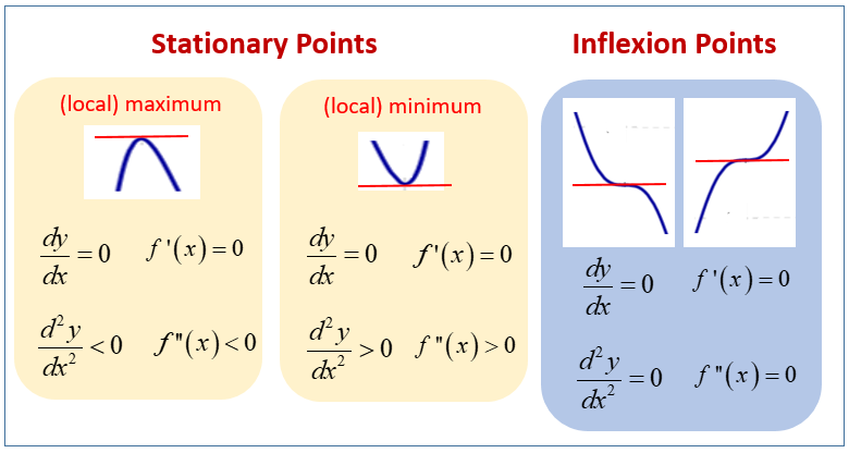
To classify a stationary point, we use the second derivative test:
- If \(f”(x_0) > 0\), the point at \(x = x_0\) is a local minimum (curve bends upwards).
- If \(f”(x_0) < 0\), the point at \(x = x_0\) is a local maximum (curve bends downwards).
- If \(f”(x_0) = 0\), the test is inconclusive — the point may be a point of inflection or require further analysis.
Using Stationary Points in Curve Sketching
When sketching a graph, stationary points are crucial:
- Find \(f'(x)\) and solve \(f'(x) = 0\) to locate stationary points.

- Use the second derivative test to classify them.
- Check end behavior (as \(x \to \pm \infty\)).
- Combine with intercepts, symmetry, and asymptotes to produce an accurate sketch.
Summary of Steps
- Differentiate \(y = f(x)\) to find \(f'(x)\).
- Solve \(f'(x) = 0\) for stationary points.
- Evaluate \(f(x)\) at these values to find coordinates.
- Use \(f”(x)\) to classify each stationary point.
- Use this information to sketch the graph.
Example:
Find the stationary points of \(y = x^3 – 3x^2 + 2\) and determine their nature.
▶️ Answer/Explanation
Step 1: Differentiate
\(y’ = 3x^2 – 6x\).
Step 2: Solve \(y’ = 0\)
\(3x^2 – 6x = 0 \implies 3x(x – 2) = 0 \implies x = 0 \text{ or } x = 2.\)
Step 3: Find coordinates
At \(x=0\): \(y = 2\). Point is \((0, 2)\).
At \(x=2\): \(y = 8 – 12 + 2 = -2\). Point is \((2, -2)\).
Step 4: Second derivative test
\(y” = 6x – 6\).
- At \(x=0\): \(y” = -6 < 0\) → local maximum at \((0, 2)\).
- At \(x=2\): \(y” = 6 > 0\) → local minimum at \((2, -2)\).
Final Answer: Local maximum at \((0, 2)\), local minimum at \((2, -2)\).
Example:
Find the stationary points of \(y = x^4 – 4x^2\) and determine their nature.
▶️ Answer/Explanation
Step 1: Differentiate
\(y’ = 4x^3 – 8x = 4x(x^2 – 2)\).
Step 2: Solve \(y’ = 0\)
\(x = 0, \; \pm \sqrt{2}\).
Step 3: Find coordinates
At \(x=0\): \(y=0\).
At \(x=\pm \sqrt{2}\): \(y = (2^2) – 4(2) = -4\). So points: \((0, 0), (\sqrt{2}, -4), (-\sqrt{2}, -4)\).
Step 4: Second derivative test
\(y” = 12x^2 – 8\).
- At \(x=0\): \(y” = -8 < 0\) → local maximum at \((0,0)\).
- At \(x=\pm \sqrt{2}\): \(y” = 12(2) – 8 = 16 > 0\) → local minima at \((\pm \sqrt{2}, -4)\).
Final Answer: Local maximum at \((0,0)\); local minima at \((\pm \sqrt{2}, -4)\).
Example:
Find the stationary points of \(y = \sin x + \cos x\) for \(0 \leq x \leq 2\pi\).
▶️ Answer/Explanation
Step 1: Differentiate
\(y’ = \cos x – \sin x\).
Step 2: Solve \(y’ = 0\)
\(\cos x = \sin x \implies \tan x = 1 \implies x = \dfrac{\pi}{4}, \dfrac{5\pi}{4}.\)
Step 3: Find coordinates
At \(x=\dfrac{\pi}{4}\): \(y = \dfrac{\sqrt{2}}{2} + \dfrac{\sqrt{2}}{2} = \sqrt{2}\).
At \(x=\dfrac{5\pi}{4}\): \(y = -\dfrac{\sqrt{2}}{2} – \dfrac{\sqrt{2}}{2} = -\sqrt{2}\).
Step 4: Second derivative test
\(y” = -\sin x – \cos x\).
- At \(x=\dfrac{\pi}{4}\): \(y” = -\dfrac{\sqrt{2}}{2} – \dfrac{\sqrt{2}}{2} = -\sqrt{2} < 0\) → local maximum at \(\left(\dfrac{\pi}{4}, \sqrt{2}\right)\).
- At \(x=\dfrac{5\pi}{4}\): \(y” = -\left(-\dfrac{\sqrt{2}}{2}\right) – \left(-\dfrac{\sqrt{2}}{2}\right) = \sqrt{2} > 0\) → local minimum at \(\left(\dfrac{5\pi}{4}, -\sqrt{2}\right)\).
Final Answer: Local maximum at \(\left(\dfrac{\pi}{4}, \sqrt{2}\right)\), local minimum at \(\left(\dfrac{5\pi}{4}, -\sqrt{2}\right)\).