Locating Roots of Equations
Many equations cannot be solved exactly (e.g., transcendental equations like \( \sin x = x/2 \)). In such cases, we can approximate the roots using: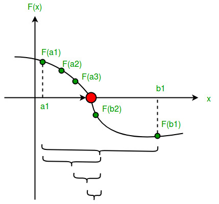
Graphical Method: Plot the functions on a graph and find where they intersect the x-axis.
Numerical Method: Look for a change of sign in the function values between two consecutive integers (or intervals). By the Intermediate Value Theorem, if \(f(a)\) and \(f(b)\) have opposite signs, then there exists at least one root between \(a\) and \(b\).
Key Steps for Sign Change Method:
- Choose consecutive integer values of \(x\).
- Evaluate the function \(f(x)\) at those values.
- If \(f(a)\) and \(f(b)\) have opposite signs, then a root lies between \(a\) and \(b\).
Example:
Find two consecutive integers between which a root of the equation \(f(x) = x^3 – 4x + 1\) lies.
▶️ Answer/Explanation
Step 1: Define the function
\(f(x) = x^3 – 4x + 1\)
Step 2: Test consecutive integer values:
\(f(0) = 0^3 – 4(0) + 1 = 1\) (positive)
\(f(1) = 1^3 – 4(1) + 1 = -2\) (negative)
Step 3: Since \(f(0) > 0\) and \(f(1) < 0\), there is a root between \(0\) and \(1\).
\(\boxed{ \text{Root lies between 0 and 1} }\)
Example:
Locate approximately a root of \(f(x) = \cos x – x\) between \(x = 0\) and \(x = 2\).
▶️ Answer/Explanation
Step 1: Define the function
\(f(x) = \cos x – x\)
Step 2: Check signs at endpoints
\(f(0) = \cos 0 – 0 = 1\) (positive)
\(f(1) = \cos 1 – 1 \approx -0.4597\) (negative)
Step 3: Since \(f(0) > 0\) and \(f(1) < 0\), a root lies between \(0\) and \(1\).
Step 4 (Graphical Consideration): Plot \(y = \cos x\) and \(y = x\). The intersection occurs near \(x \approx 0.74\).
\(\boxed{ \text{Root ≈ 0.74} }\)
Sequences of Approximations Converging to a Root
When solving equations numerically, we often cannot find an exact root. Instead, we construct a sequence of approximations that gets closer and closer to the actual root.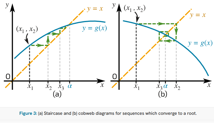
- If the true root is \(\alpha\), then we write the approximations as:
\(x_1, x_2, x_3, \dots\)
- We say that the sequence converges to \(\alpha\) if:
\(\lim_{n \to \infty} x_n = \alpha\)
- This means that as more steps are taken, the approximations get closer to the actual root.
Notation:
- \(x_1\) = first approximation
- \(x_2\) = second approximation
- \(x_3\) = third approximation, and so on
- If the sequence converges, we write:
\(x_n \to \alpha\) as \(n \to \infty\)
Example:
Use the bisection method to generate approximations to a root of \(f(x) = x^3 – 4x + 1\) between \(0\) and \(1\).
▶️ Answer/Explanation
Step 1: We already know (from sign change) that a root lies between \(0\) and \(1\).
Step 2: Take midpoint:
\(x_1 = \dfrac{0 + 1}{2} = 0.5\)
\(f(0.5) = 0.5^3 – 4(0.5) + 1 = -1.375\) (negative)
So root lies between \(0\) and \(0.5\).
Step 3: Next midpoint:
\(x_2 = \dfrac{0 + 0.5}{2} = 0.25\)
\(f(0.25) = 0.25^3 – 4(0.25) + 1 = 0.2656\) (positive)
So root lies between \(0.25\) and \(0.5\).
Step 4: Next midpoint:
\(x_3 = \dfrac{0.25 + 0.5}{2} = 0.375\)
\(f(0.375) = 0.375^3 – 4(0.375) + 1 = -0.4785\) (negative)
So root lies between \(0.25\) and \(0.375\).
Step 5: Sequence of approximations:
\(x_1 = 0.5, \; x_2 = 0.25, \; x_3 = 0.375, \dots\)
As we continue, \(x_n \to \alpha\), where \(\alpha\) is the root in \((0,1)\).
\(\boxed{ x_n \to \alpha \;\; \text{as} \;\; n \to \infty }\)
Example:
Approximate the root of \(x^2 – 3 = 0\) using the iteration \(x_{n+1} = \dfrac{3}{x_n}\), starting with \(x_1 = 1.5\).
▶️ Answer/Explanation
Step 1: True root is \(\sqrt{3} \approx 1.732\).
Step 2: Apply iteration:
\(x_1 = 1.5\)
\(x_2 = \dfrac{3}{1.5} = 2\)
\(x_3 = \dfrac{3}{2} = 1.5\)
\(x_4 = \dfrac{3}{1.5} = 2\)
Step 3: The sequence oscillates between 1.5 and 2, not converging well.
This shows that not all iterative methods converge — convergence depends on the iteration function.
\(\boxed{ \text{Iteration may converge or diverge depending on method chosen} }\)
Iterative Methods for Solving Equations
Idea of Iteration:
- Suppose we want to solve an equation \(f(x) = 0\).
- We can rearrange the equation into the form:
\(x = F(x)\)
- This leads to an iterative formula:
\(x_{n+1} = F(x_n)\)
- If the process converges, then:
\(x_n \to \alpha\) (the root of the equation)
How the Iteration Relates to the Equation:
- We start from \(f(x) = 0\).
- Rearrange into a form where \(x\) appears on both sides, e.g. \(x = F(x)\).
- The root \(\alpha\) satisfies both:
\(f(\alpha) = 0\)
\(\alpha = F(\alpha)\)
- The iteration \(x_{n+1} = F(x_n)\) generates a sequence of approximations that (hopefully) converges to \(\alpha\).
Procedure to Use Iteration:
- Choose a suitable starting value \(x_1\).
- Apply the iterative formula repeatedly:
\(x_2 = F(x_1), \; x_3 = F(x_2), \; x_4 = F(x_3), \dots\)
- Continue until two successive values agree to the required degree of accuracy (e.g., 3 decimal places).
- If values oscillate or move away from the root, the iteration fails to converge.
Key Understanding:
- Iteration works by rearranging the equation into \(x = F(x)\).
- A sequence of approximations is generated.
- If it converges, we obtain the root to the required accuracy.
- But not every rearrangement will converge – sometimes the method fails.
Example:
Solve \(x^2 – 3 = 0\) using the iteration \(x_{n+1} = \dfrac{3}{x_n}\), starting with \(x_1 = 1.5\), to 3 decimal places.
▶️ Answer/Explanation
Step 1: Rearrangement of the equation:
Original equation: \(x^2 – 3 = 0 \;\;\Rightarrow\;\; x^2 = 3 \;\;\Rightarrow\;\; x = \dfrac{3}{x}\)
So iteration: \(x_{n+1} = \dfrac{3}{x_n}\).
Step 2: Perform iterations:
\(x_1 = 1.5\)
\(x_2 = \dfrac{3}{1.5} = 2.000\)
\(x_3 = \dfrac{3}{2.000} = 1.500\)
\(x_4 = \dfrac{3}{1.500} = 2.000\)
Step 3: The sequence oscillates between 1.5 and 2.0 → it does not converge.
\(\boxed{\text{Iteration fails to converge}}\)
Example:
Solve \(x^3 + x – 1 = 0\) using the iteration \(x_{n+1} = 1 – x_n^3\), starting with \(x_1 = 0.5\), until correct to 3 decimal places.
▶️ Answer/Explanation
Step 1: Rearrangement of the equation:
\(x^3 + x – 1 = 0 \;\;\Rightarrow\;\; x = 1 – x^3\)
So iteration: \(x_{n+1} = 1 – (x_n)^3\).
Step 2: Perform iterations:
\(x_1 = 0.5\)
\(x_2 = 1 – (0.5)^3 = 1 – 0.125 = 0.875\)
\(x_3 = 1 – (0.875)^3 = 1 – 0.669 = 0.331\)
\(x_4 = 1 – (0.331)^3 = 1 – 0.036 = 0.964\)
\(x_5 = 1 – (0.964)^3 = 1 – 0.896 = 0.104\)
Step 3: The values jump around a lot. The iteration does not seem to settle.
\(\boxed{\text{Iteration fails to converge in this form}}\)
Note: If we had rearranged differently, e.g. \(x = (1 – x)^{1/3}\), the iteration may converge.