Locating Roots of an Equation Approximately
- A root of an equation \(f(x) = 0\) is a value of \(x\) where the function changes sign (from positive to negative or vice versa).
- Graphical method: Plot or sketch the graph of \(y = f(x)\) and identify points where it crosses the x-axis.
- Sign-change method: Evaluate \(f(x)\) at consecutive integers (or chosen points) and find an interval where the function changes sign. The root lies within that interval.
Steps:
- Step 1: Choose integer or convenient values of \(x\) and calculate \(f(x)\).
- Step 2: Look for a change of sign between consecutive values.
- Step 3: Conclude that a root exists in that interval.
- Step 4 (optional): Refine by checking midpoints for better approximation.
Example:
Locate a root of \(f(x) = x^3 – 5x + 1\).
▶️ Answer / Explanation
Step 1: Evaluate \(f(x)\) at consecutive integers:
\(f(0) = 0^3 – 5(0) + 1 = 1\)
\(f(1) = 1 – 5 + 1 = -3\)
Step 2: Sign changes from \(f(0) = +1\) to \(f(1) = -3\)
Step 3: Therefore, a root lies between \(x = 0\) and \(x = 1\).
Optional refinement: Evaluate at \(x = 0.2\) or \(x = 0.5\) for a better approximation.
Final Answer: Root lies in the interval \(\boxed{0 < x < 1}\)
Example:
Locate a root of \(f(x) = x^2 – 2\) using sign-change.
▶️ Answer / Explanation
Step 1: Evaluate consecutive integers:
\(f(1) = 1^2 – 2 = -1\)
\(f(2) = 2^2 – 2 = 2\)
Step 2: Sign changes from \(-1\) to \(2\)
Step 3: Therefore, a root lies between \(x = 1\) and \(x = 2\)
Optional refinement: Evaluate \(f(1.4) = 1.96 – 2 = -0.04\), \(f(1.42) = 2.0164 – 2 = 0.0164\)
Final Answer: Root lies approximately in \(\boxed{1.414 < x < 1.42}\)
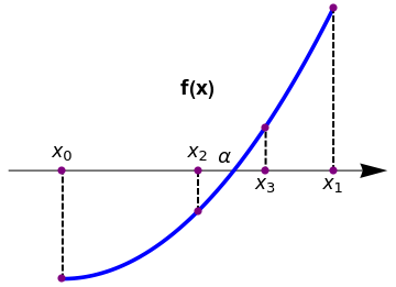
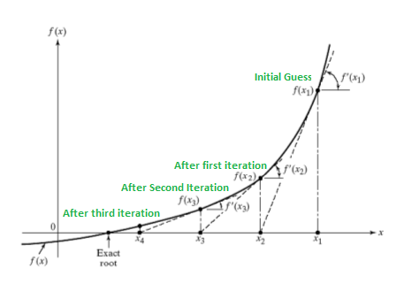
Sequences of Approximations Converging to a Root
- When a root of an equation cannot be found exactly, we can generate a sequence of approximations \(x_1, x_2, x_3, \dots\) that get closer to the true root.
- If the sequence approaches a single value as the number of iterations increases, we say the sequence converges to the root.
- Notation: \(x_n\) represents the \(n^\text{th}\) approximation, and \(\lim_{n \to \infty} x_n = r\) where \(r\) is the root.

Steps:
- Step 1: Choose a starting approximation \(x_1\) (close to where a root is expected, using sign-change or graph).
- Step 2: Generate successive approximations \(x_2, x_3, \dots\) using a suitable method (iteration formula, e.g., Newton-Raphson or fixed-point iteration).
- Step 3: Continue until successive approximations differ by less than a desired tolerance, indicating convergence.
Example:
Consider finding a root of \(x^2 – 2 = 0\) using the iterative formula \(x_{n+1} = \frac{1}{2} \left(x_n + \frac{2}{x_n}\right)\).
▶️ Answer / Explanation
Step 1: Choose initial approximation \(x_1 = 1.5\)
Step 2: Apply the iteration formula:
\(x_2 = \frac{1}{2} \left(1.5 + \frac{2}{1.5}\right) = \frac{1}{2} (1.5 + 1.3333) = 1.4167\)
\(x_3 = \frac{1}{2} \left(1.4167 + \frac{2}{1.4167}\right) \approx 1.4142\)
\(x_4 = \frac{1}{2} \left(1.4142 + \frac{2}{1.4142}\right) \approx 1.4142\)
Step 3: Successive approximations are converging to \(\sqrt{2} \approx 1.4142\)
Final Answer: The sequence \(\{x_n\}\) converges to the root \(\boxed{r = \sqrt{2} \approx 1.4142}\)
Example:
Using a fixed-point iteration to solve \(x = \cos x\) with \(x_{n+1} = \cos x_n\) and \(x_1 = 0.5\)
▶️ Answer / Explanation
\(x_2 = \cos 0.5 \approx 0.8776\)
\(x_3 = \cos 0.8776 \approx 0.6390\)
\(x_4 = \cos 0.6390 \approx 0.8027\)
\(x_5 = \cos 0.8027 \approx 0.6947\)
\(x_6 = \cos 0.6947 \approx 0.7682\)
Step 3: The sequence oscillates and gradually converges to approximately \(x \approx 0.7391\)
Final Answer: \(\boxed{r \approx 0.7391}\)
Solving Equations Using Simple Iteration
- A simple iterative formula is of the form \(x_{n+1} = F(x_n)\), where each successive approximation \(x_{n+1}\) is computed from the previous one \(x_n\).
- The root of the equation corresponds to a value \(r\) satisfying \(r = F(r)\).
- The method requires a starting value \(x_1\) and repeated application of the iteration until the approximations converge to the desired accuracy.
- Note: Iteration may fail to converge if the chosen formula or starting value is unsuitable.
Steps:
- Step 1: Rewrite the equation \(f(x) = 0\) in the form \(x = F(x)\).
- Step 2: Choose an initial approximation \(x_1\), preferably near where the root is expected (from a graph or sign-change method).
- Step 3: Apply the iteration formula \(x_{n+1} = F(x_n)\) repeatedly.
- Step 4: Continue until \(|x_{n+1} – x_n|\) is smaller than a given tolerance (desired degree of accuracy).
- Step 5: Report the root as the final approximation within the prescribed accuracy.
Example:
Solve \(x^3 + x – 1 = 0\) using iteration formula \(x_{n+1} = 1 – x_n^3\) starting with \(x_1 = 0.5\) to 3 decimal places.
▶️ Answer / Explanation
Step 1: Iteration formula given: \(x_{n+1} = 1 – x_n^3\)
Step 2: Apply iteration:
\(x_1 = 0.5\)
\(x_2 = 1 – (0.5)^3 = 1 – 0.125 = 0.875\)
\(x_3 = 1 – (0.875)^3 = 1 – 0.6699 = 0.3301\)
\(x_4 = 1 – (0.3301)^3 \approx 1 – 0.0359 = 0.9641\)
…sequence oscillates and does not converge quickly
Observation: Iteration may fail to converge for this rearrangement.
Example:
Solve \(x^3 – x – 2 = 0\) using \(x_{n+1} = \sqrt[3]{x_n + 2}\) starting with \(x_1 = 1.5\) to 3 decimal places.
▶️ Answer / Explanation
Step 1: Iteration formula given: \(x_{n+1} = \sqrt[3]{x_n + 2}\)
Step 2: Apply iteration:
\(x_1 = 1.5\)
\(x_2 = \sqrt[3]{1.5 + 2} = \sqrt[3]{3.5} \approx 1.518\)
\(x_3 = \sqrt[3]{1.518 + 2} = \sqrt[3]{3.518} \approx 1.522\)
\(x_4 = \sqrt[3]{1.522 + 2} = \sqrt[3]{3.522} \approx 1.523\)
Step 3: \(|x_4 – x_3| \approx 0.001 < 0.0015\) → desired accuracy reached
Final Answer: Root \(\boxed{x \approx 1.523}\)
Example 3:
Solve \(x = \cos x\) using iteration formula \(x_{n+1} = \cos x_n\) starting with \(x_1 = 0.5\) to 4 decimal places.
▶️ Answer / Explanation
\(x_1 = 0.5\)
\(x_2 = \cos 0.5 \approx 0.8776\)
\(x_3 = \cos 0.8776 \approx 0.6390\)
\(x_4 = \cos 0.6390 \approx 0.8027\)
\(x_5 = \cos 0.8027 \approx 0.6947\)
\(x_6 = \cos 0.6947 \approx 0.7682\)
Continue iteration until \(|x_{n+1} – x_n| < 0.0001\)
Final Answer: Root \(\boxed{x \approx 0.7391}\)