Rate of Change and Differential Equations
In many real-world problems, a quantity changes over time (or another variable), and the rate of change of this quantity can often be expressed as a differential equation. A differential equation is an equation that relates a function to its derivatives.
Basic Concept
Let \(y\) be a quantity that depends on time \(t\). The rate of change of \(y\) with respect to \(t\) is written as \(\dfrac{dy}{dt}\).
If the rate of change is proportional to the quantity itself, we can write:
\(\dfrac{dy}{dt} \propto y\)
Here, the symbol \(\propto\) means “proportional to”.
Introducing a constant of proportionality \(k\), we write the differential equation as:
\(\dfrac{dy}{dt} = k y\)
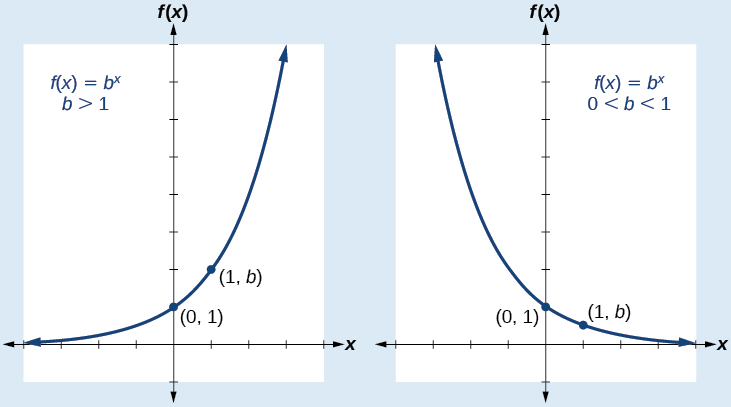
- \(k > 0\) indicates growth.
- \(k < 0\) indicates decay.
Other Types of Rate of Change
Rate of change proportional to a function of time \(t\):
\(\dfrac{dy}{dt} = k f(t)\)
Rate of change proportional to the difference from a limiting value \(y_0\):
\(\dfrac{dy}{dt} = k (y_0 – y)\)
Rate of change inversely proportional to the quantity:
\(\dfrac{dy}{dt} \propto \dfrac{1}{y} \implies \dfrac{dy}{dt} = \dfrac{k}{y}\)
Formulating a Differential Equation from a Statement
- Step 1: Identify the quantity that changes and the independent variable (usually time \(t\)).
- Step 2: Express the rate of change (derivative) of the quantity in words.
- Step 3: Introduce a constant of proportionality \(k\) if the change is proportional to a quantity.
- Step 4: Write the corresponding differential equation.
Example:
The rate of growth of a bacteria population \(P\) is proportional to its current population.
▶️ Answer/Explanation
Step 1: Quantity changing: \(P\), independent variable: \(t\)
Step 2: Rate of change is proportional to the population: \(\dfrac{dP}{dt} \propto P\)
Step 3: Introduce constant \(k\): \(\dfrac{dP}{dt} = k P\)
Example:
The cooling of an object is proportional to the difference between its temperature \(T\) and the ambient temperature \(T_a\).
▶️ Answer/Explanation
Step 1: Quantity changing: \(T\), independent variable: \(t\)
Step 2: Rate of change: \(\dfrac{dT}{dt} \propto (T_a – T)\)
Step 3: Introduce constant \(k\): \(\dfrac{dT}{dt} = k (T_a – T)\)
Example:
The rate of spread of a rumor is inversely proportional to the number of people who already know it \(R\).
▶️ Answer/Explanation
Step 1: Quantity changing: \(R\), independent variable: \(t\)
Step 2: Rate of change: \(\dfrac{dR}{dt} \propto \dfrac{1}{R}\)
Step 3: Introduce constant \(k\): \(\dfrac{dR}{dt} = \dfrac{k}{R}\)
Solving First-Order Separable Differential Equations
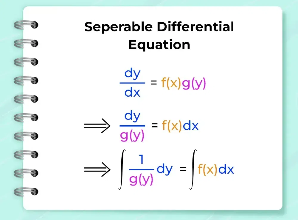
A first-order differential equation is said to be separable if it can be written in the form:
\(\dfrac{dy}{dx} = f(x) g(y)\)
Here, the variables \(x\) and \(y\) can be separated so that all terms involving \(y\) are on one side and all terms involving \(x\) are on the other:
\(\dfrac{1}{g(y)} dy = f(x) dx\)
Once separated, both sides can be integrated to find the general solution.
Step-by-Step Method
- Step 1: Start with the differential equation in the form \(\dfrac{dy}{dx} = f(x) g(y)\).
- Step 2: Rearrange to separate the variables: \(\dfrac{1}{g(y)} dy = f(x) dx\).
- Step 3: Integrate both sides:
\(\displaystyle \int \dfrac{1}{g(y)} dy = \int f(x) dx + C\)
where \(C\) is the constant of integration.
- Step 4: Solve for \(y\) explicitly if possible.
- Step 5: Apply any initial conditions to determine the particular solution if given.
Common Integration Techniques (from Topic 3.5)
- Direct integration: \(\displaystyle \int k \, dx = kx + C\)
- Power rule: \(\displaystyle \int x^n dx = \dfrac{x^{n+1}}{n+1} + C, \ n \neq -1\)
- Reciprocal linear function: \(\displaystyle \int \dfrac{1}{ax + b} dx = \dfrac{1}{a} \ln |ax + b| + C\)
- Exponential function: \(\displaystyle \int e^{ax+b} dx = \dfrac{1}{a} e^{ax+b} + C\)
- Trigonometric functions:
\(\displaystyle \int \sin(ax) dx = -\dfrac{1}{a} \cos(ax) + C\)
\(\displaystyle \int \cos(ax) dx = \dfrac{1}{a} \sin(ax) + C\)
Example 1:
Find the general solution of \(\dfrac{dy}{dx} = xy^2\).
▶️ Answer/Explanation
Step 1: Separate variables:
\(\dfrac{1}{y^2} dy = x dx\)
Step 2: Integrate both sides:
\(\displaystyle \int y^{-2} dy = \int x dx \implies -y^{-1} = \dfrac{x^2}{2} + C\)
Step 3: Solve for \(y\):
\(\boxed{y = -\dfrac{1}{\dfrac{x^2}{2} + C}}\)
Example 2:
Find the general solution of \(\dfrac{dy}{dx} = \dfrac{y}{x}\).
▶️ Answer/Explanation
Step 1: Separate variables:
\(\dfrac{1}{y} dy = \dfrac{1}{x} dx\)
Step 2: Integrate both sides:
\(\displaystyle \int \dfrac{1}{y} dy = \int \dfrac{1}{x} dx \implies \ln |y| = \ln |x| + C\)
Step 3: Solve for \(y\):
\(\boxed{y = K x, \text{ where } K = e^C}\)
Example 3:
Find the general solution of \(\dfrac{dy}{dx} = e^x \sin y\).
▶️ Answer/Explanation
Step 1: Separate variables:
\(\dfrac{1}{\sin y} dy = e^x dx\)
Step 2: Integrate both sides (use \(\int \csc y dy = \ln|\tan(y/2)| + C\)):
\(\ln |\tan(y/2)| = e^x + C\)
Step 3: Solve for \(y\) implicitly:
\(\boxed{y = 2 \arctan\big(K e^{e^x}\big), \ K = e^C}\)
Finding a Particular Solution Using an Initial Condition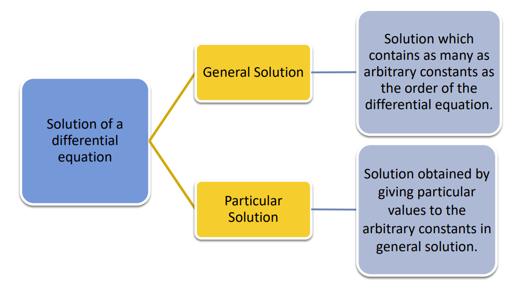
After finding the general solution of a differential equation, we often have additional information called an initial condition. This is usually of the form:
\(y(x_0) = y_0\)
where \(y_0\) is the value of the function at \(x = x_0\). We use this to determine the constant of integration \(C\) and obtain a particular solution.
Step-by-Step Method
- Step 1: Solve the differential equation to get the general solution:
\(y = f(x) + C\)
- Step 2: Substitute the initial condition \(x = x_0, y = y_0\) into the general solution.
- Step 3: Solve for the constant \(C\).
- Step 4: Substitute \(C\) back into the general solution to get the particular solution.
Example:
Solve \(\dfrac{dy}{dx} = xy^2\) with the initial condition \(y(0) = 2\).
▶️ Answer/Explanation
Step 1: General solution (from previous example):
\(\displaystyle y = -\dfrac{1}{\dfrac{x^2}{2} + C}\)
Step 2: Apply the initial condition \(y(0) = 2\):
\(2 = -\dfrac{1}{0 + C} \implies C = -\dfrac{1}{2}\)
Step 3: Substitute \(C\) into the general solution:
\(\displaystyle \boxed{y = -\dfrac{1}{\dfrac{x^2}{2} – \dfrac{1}{2}}} = -\dfrac{1}{\dfrac{x^2 – 1}{2}} = -\dfrac{2}{x^2 – 1}\)
Example:
Solve \(\dfrac{dy}{dx} = \dfrac{y}{x}\) with \(y(1) = 3\).
▶️ Answer/Explanation
Step 1: General solution (from previous example):
\(y = K x\)
Step 2: Apply the initial condition \(y(1) = 3\):
\(3 = K \cdot 1 \implies K = 3\)
Step 3: Particular solution:
\(\boxed{y = 3x}\)
Example:
Solve \(\dfrac{dy}{dx} = e^x \sin y\) with \(y(0) = \pi/2\).
▶️ Answer/Explanation
Step 1: General solution (from previous example):
\(\ln |\tan(y/2)| = e^x + C\)
Step 2: Apply initial condition \(y(0) = \pi/2\):
\(\ln |\tan(\pi/4)| = e^0 + C \implies 0 = 1 + C \implies C = -1\)
Step 3: Particular solution:
\(\boxed{\ln |\tan(y/2)| = e^x – 1}\)
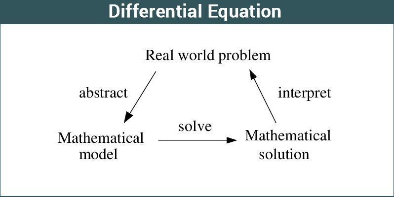
Interpreting the Solution of a Differential Equation in Context
When a differential equation is used to model a real-world situation, the solution provides information about how the quantity of interest changes with respect to the independent variable (often time). Interpretation means connecting the mathematical solution back to the physical, biological, or economic context.
General Steps
- Step 1: Identify the quantity being modeled (e.g., population, temperature, concentration, speed).
- Step 2: Identify the independent variable (usually time \(t\)).
- Step 3: Analyze the general solution to understand the behavior of the system:
- Growth or decay: Is the quantity increasing or decreasing over time?
- Equilibrium: Does the solution approach a limiting value as \(t \to \infty\)?
- Rate of change: How does the constant of proportionality \(k\) affect the speed of change?
- Step 4: Use a particular solution (if an initial condition is given) to make specific predictions.
Key Points to Consider
- Positive vs negative constants: \(k>0\) often indicates growth, \(k<0\) indicates decay.
- Long-term behavior: Examine what happens as \(t \to \infty\) (e.g., population approaches a maximum, temperature approaches ambient).
- Initial condition relevance: Shows the starting point of the system and ensures the model matches the situation.
Example:
A bacteria population \(P(t)\) satisfies \(\dfrac{dP}{dt} = 0.5 P\) with initial population \(P(0) = 100\).
▶️ Answer/Explanation
Step 1: Solve the differential equation:
General solution: \(P = P_0 e^{0.5 t}\)
Particular solution using initial condition \(P(0)=100\):
\(P = 100 e^{0.5 t}\)
Step 2: Interpret in context:
- The population grows exponentially over time because \(k=0.5>0\).
- Initially \(P = 100\) at \(t=0\).
- As \(t\) increases, the population increases without bound (no limiting factor in the model).
Example:
The cooling of a hot object is modeled by \(\dfrac{dT}{dt} = -0.1 (T – 25)\) with initial temperature \(T(0) = 85^\circ\)C, where \(T_a = 25^\circ\)C is ambient temperature.
▶️ Answer/Explanation
Step 1: Solve the differential equation:
General solution: \(T – 25 = C e^{-0.1 t}\)
Use initial condition \(T(0)=85\):
\(85-25 = C \implies C = 60\)
Particular solution: \(T = 25 + 60 e^{-0.1 t}\)
Step 2: Interpret in context:
- At \(t=0\), \(T = 85^\circ\)C.
- As \(t \to \infty\), \(e^{-0.1 t} \to 0\), so \(T \to 25^\circ\)C, the ambient temperature.
- The negative rate constant indicates cooling rather than heating.
Example:
A tank contains salt solution. The concentration of salt \(y(t)\) decreases according to \(\dfrac{dy}{dt} = -0.2 y\), with \(y(0) = 50\) g.
▶️ Answer/Explanation
Step 1: Solve the differential equation:
General solution: \(y = C e^{-0.2 t}\)
Use initial condition \(y(0) = 50\): \(C = 50\)
Particular solution: \(y = 50 e^{-0.2 t}\)
Step 2: Interpret in context:
- The salt concentration decreases exponentially over time.
- As \(t \to \infty\), \(y \to 0\), meaning the tank eventually becomes salt-free.
- The rate constant \(0.2\) determines how quickly the concentration decreases.