Normal Distribution
A continuous random variable \(X\) is said to follow a normal distribution if its probability density function has the form: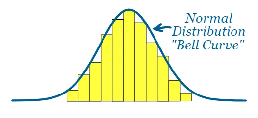
\( f(x) = \dfrac{1}{\sigma \sqrt{2\pi}} \, e^{-\frac{(x-\mu)^2}{2\sigma^2}} \), for \( -\infty < x < \infty \)
- \(\mu\) = mean of the distribution
- \(\sigma\) = standard deviation of the distribution
Notation: \( X \sim N(\mu, \sigma^2) \)
Key properties: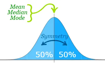
- The curve is symmetric about \(x = \mu\)
- The total area under the curve is 1
- Approximately 68% of values lie within \( \mu \pm \sigma \), 95% within \( \mu \pm 2\sigma \), 99.7% within \( \mu \pm 3\sigma \)
Standard Normal Distribution:
- Let \( Z = \dfrac{X-\mu}{\sigma} \), then \( Z \sim N(0, 1) \)
- Normal distribution tables give probabilities for \( P(Z \le z) \)
- Probabilities for other events can be found using symmetry and complements:
\( P(Z \ge z) = 1 – P(Z \le z), \quad P(a \le Z \le b) = P(Z \le b) – P(Z \le a) \)
Sketches of the normal curve may be used to illustrate: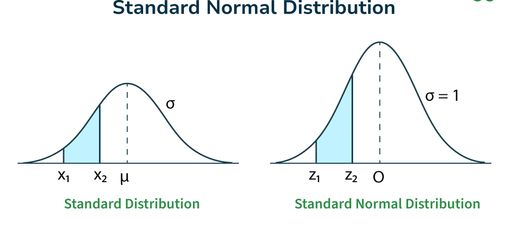
- Mean and standard deviations
- Probability regions (shaded area under the curve)
Practical use:
- Modeling heights, test scores, measurement errors, and other naturally occurring continuous data
- Finding probabilities for ranges of values using tables or software
Example:
The heights of adult men are approximately normally distributed with mean 175 cm and standard deviation 8 cm. Find the probability that a randomly chosen man is taller than 183 cm.
▶️ Answer/Explanation
Let \(X \sim N(175, 8^2)\)
Standardize: \( Z = \dfrac{X-\mu}{\sigma} = \dfrac{183-175}{8} = 1 \)
From standard normal table: \( P(Z \le 1) = 0.8413 \)
So, \( P(X > 183) = P(Z > 1) = 1 – 0.8413 = 0.1587 \)
Final Answer: \(\boxed{0.1587}\)
Example:
Using the same data, find the probability that a randomly chosen man is between 167 cm and 183 cm.
▶️ Answer/Explanation
Standardize lower value: \( Z_1 = \dfrac{167-175}{8} = -1 \)
Standardize upper value: \( Z_2 = \dfrac{183-175}{8} = 1 \)
From table: \( P(Z \le 1) = 0.8413, \quad P(Z \le -1) = 0.1587 \)
Probability between: \( P(167 \le X \le 183) = P(Z_2) – P(Z_1) = 0.8413 – 0.1587 = 0.6826 \)
Final Answer: \(\boxed{0.6826}\)
Normal Distribution Problems with \(X \sim N(\mu, \sigma^2)\)
When a variable \(X\) is normally distributed, probabilities can be found by standardising: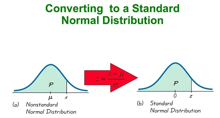
\( Z = \dfrac{X – \mu}{\sigma} \)
- This converts \(X\) to a standard normal variable \(Z \sim N(0,1)\), so that standard normal tables can be used.
Finding probabilities \(P(X > x_1)\) or related
- Step 1: Standardise: \( Z = \dfrac{x_1 – \mu}{\sigma} \)
- Step 2: Use standard normal table to find \(P(Z \le z)\)
- Step 3: Apply complement if needed: \( P(X > x_1) = P(Z > z) = 1 – P(Z \le z) \)
Finding \(x_1\) or a relationship between \(x_1, \mu, \sigma\)
- Step 1: Identify the probability: e.g., \( P(X > x_1) = 0.05 \)
- Step 2: Convert to standard normal probability: \( P(Z > z_1) = 0.05 \)
- Step 3: Find \(z_1\) from standard normal table: \( z_1 = 1.645 \) (for upper 5%)
- Step 4: Use \( Z = \dfrac{x_1 – \mu}{\sigma} \) to solve for \(x_1\) or relate it to \(\mu, \sigma\)
- For Complete Z Table : Link
Example:
A variable \(X \sim N(100, 16)\). Find \(P(X > 108)\).
▶️ Answer/Explanation
Step 1: Standardise
\( Z = \dfrac{X – \mu}{\sigma} = \dfrac{108 – 100}{4} = 2 \)
Step 2: Find \(P(Z \le 2)\) from table: \(0.9772\)
Step 3: Apply complement: \( P(X > 108) = P(Z > 2) = 1 – 0.9772 = 0.0228 \)
Final Answer: \(\boxed{0.0228}\)
Example:
For a variable \(X \sim N(50, 25)\), find \(x_1\) such that \(P(X > x_1) = 0.05\).
▶️ Answer/Explanation
Step 1: Convert probability to standard normal: \( P(Z > z_1) = 0.05 \)
Step 2: From standard normal table: \( z_1 = 1.645 \)
Step 3: Use standardisation formula:
\( z_1 = \dfrac{x_1 – \mu}{\sigma} \implies 1.645 = \dfrac{x_1 – 50}{5} \)
Step 4: Solve for \(x_1\): \( x_1 = 1.645 \cdot 5 + 50 = 58.225 \)
Final Answer: \(\boxed{58.23}\)
Normal Approximation to the Binomial Distribution
A binomial distribution \(X \sim B(n, p)\) can be approximated by a normal distribution \(N(\mu, \sigma^2)\) when \(n\) is sufficiently large.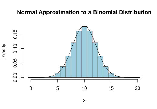
Conditions for approximation:
- Number of trials \(n\) is large enough so that both \(np > 5\) and \(nq > 5\), where \(q = 1-p\).
- This ensures the binomial distribution is not too skewed and the approximation is reasonable.
Parameters of approximating normal distribution:
- Mean: \( \mu = np \)
- Variance: \( \sigma^2 = npq \)
- Standard deviation: \( \sigma = \sqrt{npq} \)
Continuity correction:
- Because a binomial variable is discrete and normal is continuous, adjust the boundary by 0.5 when approximating probabilities.
- Example: \( P(X \le k) \approx P(Y \le k + 0.5) \), \( P(X \ge k) \approx P(Y \ge k – 0.5) \), where \(Y \sim N(np, npq)\).
Steps to use the approximation:
- Step 1: Check conditions \(np > 5\) and \(nq > 5\)
- Step 2: Calculate \(\mu = np\) and \(\sigma = \sqrt{npq}\)
- Step 3: Apply continuity correction to the desired probability
- Step 4: Standardise to \( Z = \dfrac{X – \mu}{\sigma} \) (including the correction)
- Step 5: Use standard normal table to find probability
Example:
A fair coin is tossed 100 times. Use the normal approximation to find the probability of getting at most 60 heads.
▶️ Answer/Explanation
Step 1: Check conditions
\( n = 100, p = 0.5, q = 0.5 \)
\( np = 100 \cdot 0.5 = 50 > 5, \quad nq = 100 \cdot 0.5 = 50 > 5 \)
Step 2: Parameters of approximating normal:
\( \mu = np = 50, \quad \sigma = \sqrt{npq} = \sqrt{100 \cdot 0.5 \cdot 0.5} = 5 \)
Step 3: Apply continuity correction: \( P(X \le 60) \approx P(Y \le 60.5) \)
Step 4: Standardise:
\( Z = \dfrac{60.5 – 50}{5} = 2.1 \)
Step 5: Use standard normal table: \( P(Z \le 2.1) = 0.9821 \)
Final Answer: \(\boxed{0.9821}\)