Poisson Distribution
A random variable \(X\) follows a Poisson distribution if it counts the number of events occurring in a fixed interval of time or space, given that the events occur independently and at a constant average rate.
Notation:
\(X \sim \text{Po}(\lambda)\), where \(\lambda > 0\) is the mean number of events in the interval.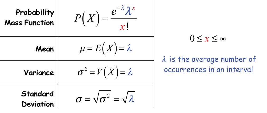
Probability mass function (pmf):
\( P(X = k) = \dfrac{\lambda^k e^{-\lambda}}{k!}, \quad k = 0, 1, 2, \dots \)
Mean and variance:
\( E(X) = \lambda, \quad \text{Var}(X) = \lambda \)
Key properties:
- Used for rare events in a large population or interval
- Events occur independently
- Interval size must be fixed
Practical examples: number of phone calls at a call center per hour, number of typing errors per page, number of accidents at a junction per month.
Example:
The average number of cars passing a checkpoint in an hour is 3. Find the probability that exactly 5 cars pass in one hour.
▶️ Answer/Explanation
Here \(X \sim \text{Po}(\lambda=3)\)
\( P(X = 5) = \dfrac{3^5 e^{-3}}{5!} = \dfrac{243 \cdot e^{-3}}{120} \approx 0.1008 \)
Final Answer: \(\boxed{0.1008}\)
Example:
The average number of typing errors on a page is 2. Find the probability that there is at least 1 error on a page.
▶️ Answer/Explanation
Here \(X \sim \text{Po}(\lambda=2)\)
\( P(X \ge 1) = 1 – P(X=0) \)
\( P(X=0) = \dfrac{2^0 e^{-2}}{0!} = e^{-2} \approx 0.1353 \)
\( P(X \ge 1) = 1 – 0.1353 = 0.8647 \)
Final Answer: \(\boxed{0.8647}\)
Relevance of the Poisson Distribution
The Poisson distribution is used to model the number of times an event occurs in a fixed interval of time, space, or other continuous domain.
Key conditions for using the Poisson model:
- Events occur independently of each other.
- The average rate of occurrence, \(\lambda\), is constant over the interval.
- The probability of more than one event occurring in an infinitesimally small sub-interval is negligible.

Notation:
\(X \sim \text{Po}(\lambda)\), where \(X\) is the number of events in the interval.
Probability of observing exactly \(k\) events in the interval:
\( P(X = k) = \dfrac{\lambda^k e^{-\lambda}}{k!}, \quad k = 0, 1, 2, \dots \)
Mean and variance:
\( E(X) = \lambda, \quad \text{Var}(X) = \lambda \)
Applications include:
- Number of phone calls received at a call center per hour
- Number of typing errors per page
- Number of accidents at a traffic junction per month
- Number of decay events from a radioactive source per unit time
The Poisson model is particularly useful when:
- The total number of trials is large
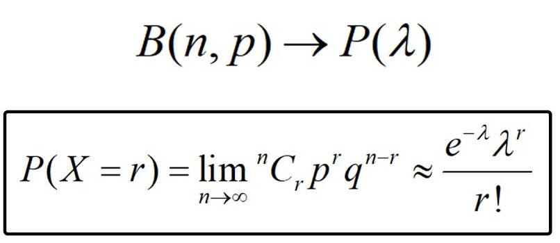
- The probability of a single event in each trial is small
- This is the limiting case of a binomial distribution \(B(n, p)\) as \(n \to \infty\) and \(p \to 0\) such that \(np = \lambda\)
Example:
The average number of emails received by a manager per hour is 4. Using a Poisson model, find the probability that exactly 6 emails are received in an hour.
▶️ Answer/Explanation
Let \(X \sim \text{Po}(\lambda = 4)\)
\( P(X = 6) = \dfrac{4^6 e^{-4}}{6!} = \dfrac{4096 \cdot e^{-4}}{720} \approx 0.1042 \)
Final Answer: \(\boxed{0.1042}\)
Example:
On average, 2 customers arrive at a shop per 10-minute interval. Using a Poisson model, calculate the probability that no customer arrives in a 10-minute interval.
▶️ Answer/Explanation
Let \(X \sim \text{Po}(\lambda = 2)\)
\( P(X = 0) = \dfrac{2^0 e^{-2}}{0!} = e^{-2} \approx 0.1353 \)
Final Answer: \(\boxed{0.1353}\)
Poisson Approximation to the Binomial Distribution
The binomial distribution \(X \sim B(n, p)\) can be approximated by a Poisson distribution when:
- The number of trials \(n\) is large (typically \(n > 50\))
- The probability of success \(p\) is small
- The expected number of successes \(np\) is moderate (typically \(np < 5\))
In such cases, the binomial \(B(n, p)\) can be approximated by \( \text{Po}(\lambda) \) with:
\( \lambda = np \)
Probability formula using the Poisson approximation:
\( P(X = k) \approx \dfrac{\lambda^k e^{-\lambda}}{k!}, \quad k = 0, 1, 2, \dots \)
- This is useful when exact binomial calculations are cumbersome due to large \(n\).
- Applications include counting rare events in a large number of trials, e.g., number of defective items in a large batch, number of accidents in a day, or number of network failures in a large system.
Example:
A factory produces 2000 items per day. The probability that an item is defective is 0.002. Use a Poisson approximation to find the probability that exactly 3 items are defective in a day.
▶️ Answer/Explanation
Step 1: Check conditions
\( n = 2000 > 50, \quad p = 0.002 \text{ small}, \quad np = 2000 \cdot 0.002 = 4 < 5 \) → Poisson approximation appropriate
Step 2: Use Poisson approximation: \( \lambda = np = 4 \)
Step 3: Calculate probability:
\( P(X = 3) \approx \dfrac{4^3 e^{-4}}{3!} = \dfrac{64 e^{-4}}{6} \approx 0.1954 \)
Final Answer: \(\boxed{0.1954}\)
Example:
A website receives 1000 hits per day. The probability that a hit is from a specific country is 0.003. Use a Poisson approximation to find the probability that exactly 2 hits are from that country in a day.
▶️ Answer/Explanation
Step 1: Check conditions
\( n = 1000 > 50, \quad p = 0.003 \text{ small}, \quad np = 1000 \cdot 0.003 = 3 < 5 \) → Poisson approximation appropriate
Step 2: Use Poisson approximation: \( \lambda = np = 3 \)
Step 3: Calculate probability:
\( P(X = 2) \approx \dfrac{3^2 e^{-3}}{2!} = \dfrac{9 e^{-3}}{2} \approx 0.2240 \)
Final Answer: \(\boxed{0.2240}\)
Normal Approximation to the Poisson Distribution
A Poisson distribution \(X \sim \text{Po}(\lambda)\) can be approximated by a normal distribution when the mean \(\lambda\) is large.
Condition for approximation: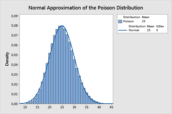
- \(\lambda > 15\) (approximately)
- This ensures the Poisson distribution is sufficiently symmetric for the normal approximation to be reasonable.
Parameters of the approximating normal distribution:
Mean: \( \mu = \lambda \)
Variance: \( \sigma^2 = \lambda \), Standard deviation: \( \sigma = \sqrt{\lambda} \)
Continuity correction:
- Since the Poisson variable is discrete and normal is continuous, adjust the boundary by 0.5 when approximating probabilities.
- Example: \( P(X \le k) \approx P(Y \le k + 0.5) \), \( P(X \ge k) \approx P(Y \ge k – 0.5) \), where \(Y \sim N(\lambda, \lambda)\).
Steps to use the approximation:
- Step 1: Check that \(\lambda > 15\)
- Step 2: Use \( \mu = \lambda, \sigma = \sqrt{\lambda} \)
- Step 3: Apply continuity correction to the desired probability
- Step 4: Standardise using \( Z = \dfrac{X – \mu}{\sigma} \)
- Step 5: Use standard normal table to find probability
Example:
The average number of calls received by a call center per day is 20. Use a normal approximation to find the probability that at most 25 calls are received in a day.
▶️ Answer/Explanation
Step 1: Check condition: \(\lambda = 20 > 15\) → approximation appropriate
Step 2: Parameters of approximating normal:
\( \mu = 20, \quad \sigma = \sqrt{20} \approx 4.472 \)
Step 3: Apply continuity correction:
\( P(X \le 25) \approx P(Y \le 25.5) \)
Step 4: Standardise:
\( Z = \dfrac{25.5 – 20}{4.472} \approx 1.23 \)
Step 5: Use standard normal table: \( P(Z \le 1.23) \approx 0.8907 \)
Final Answer: \(\boxed{0.8907}\)
Example:
The number of typing errors on a long document is Poisson distributed with mean 30. Use a normal approximation to find the probability that there are at least 35 errors.
▶️ Answer/Explanation
Step 1: Check condition: \(\lambda = 30 > 15\) → approximation appropriate
Step 2: Parameters of approximating normal:
\( \mu = 30, \quad \sigma = \sqrt{30} \approx 5.477 \)
Step 3: Apply continuity correction:
\( P(X \ge 35) \approx P(Y \ge 34.5) \)
Step 4: Standardise:
\( Z = \dfrac{34.5 – 30}{5.477} \approx 0.82 \)
Step 5: Use standard normal table: \( P(Z \ge 0.82) = 1 – 0.7939 = 0.2061 \)
Final Answer: \(\boxed{0.2061}\)