Sample and Population
A population is the entire set of individuals, items, or measurements under study. For example, the population could be all students in a school, all voters in a country, or all manufactured light bulbs in a factory.
A sample is a smaller group selected from the population, intended to represent the population. For example, a group of 50 students chosen from the school to represent the views of all students.
Sampling is used because it is often impractical or impossible to collect data from the entire population (too large, expensive, or time-consuming).
Necessity of Randomness
A sample should be chosen at random so that every individual has an equal chance of being selected.
Randomness ensures the sample is unbiased and more likely to be representative of the population.
Without randomness, results can be misleading or inaccurate, because some groups may be over- or under-represented.
Unsatisfactory Sampling Methods (with reasons)
- Choosing friends or people nearby: This may only represent a certain group and not the entire population → biased.
- Voluntary responses: Only people interested might respond (e.g. online surveys) → not representative.
- Taking the first items available: May not reflect the whole population (e.g. interviewing only morning shoppers in a supermarket).
Use of Random Numbers
Random numbers can be generated (using a calculator, computer, or random number tables) to select individuals in a population.
Example: If a school has 500 students, number them from 1 to 500. Then use random numbers to pick, say, 30 students for the sample. This avoids bias and ensures fairness.
Example:
A teacher wants to find out how much time students in her school spend on homework. The school has 600 students. She decides to ask the first 30 students who arrive at school one morning.
▶️ Answer/Explanation
This method is unsatisfactory because the first 30 students are not a random sample. They may all be early arrivers, who could be more organised or more studious than average.
A better method is to number all 600 students and use random numbers to select 30 students. This way, every student has an equal chance of being chosen, and the sample is more representative of the population.
Example:
A company wants to know how many hours people watch TV each week. They post a survey online and ask for volunteers to fill it in.
▶️ Answer/Explanation
This method is unsatisfactory because only those who are interested in the survey (perhaps heavy TV watchers) are likely to respond. The sample is not random and may not represent the population.
A better method would be to select people randomly from the population (for example, from a list of addresses or phone numbers) and then ask them.
Sample Mean Distribution when \(X\) is Normal
Suppose the population random variable \(X\) follows a Normal distribution:
\(X \sim N(\mu, \sigma^2)\)
If we take a random sample of size \(n\), then the sample mean is:
\(\overline{X} = \dfrac{X_1 + X_2 + \dots + X_n}{n}\)
A key fact: If \(X\) is normal, then \(\overline{X}\) is also normally distributed (no matter what \(n\) is).
The distribution of \(\overline{X}\) is:
\(\overline{X} \sim N\!\Big(\mu, \dfrac{\sigma^2}{n}\Big)\)
This means:
- The mean of \(\overline{X}\) is the same as the population mean \(\mu\).
- The variance of \(\overline{X}\) is reduced by a factor of \(n\): \(\dfrac{\sigma^2}{n}\).
- The standard deviation of \(\overline{X}\), called the standard error, is \(\dfrac{\sigma}{\sqrt{n}}\).
Example:
The lifetimes of batteries are normally distributed with mean \(\mu = 50\) hours and standard deviation \(\sigma = 8\) hours. A random sample of \(n = 16\) batteries is taken. Find the distribution of the sample mean \(\overline{X}\).
▶️ Answer/Explanation
We know:
\(\overline{X} \sim N\!\Big(\mu, \dfrac{\sigma^2}{n}\Big)\)
So, \(\mu = 50\), \(\sigma^2 = 8^2 = 64\), \(n = 16\).
\(\text{Var}(\overline{X}) = \dfrac{64}{16} = 4\)
\(\text{SE} = \sqrt{4} = 2\)
Therefore:
\(\boxed{\overline{X} \sim N(50, 4)}\)
Example:
The weights of packets of sugar are normally distributed with mean \(\mu = 1 \ \text{kg}\) and standard deviation \(\sigma = 0.05 \ \text{kg}\). A random sample of \(n = 25\) packets is chosen. Find the probability that the sample mean weight is greater than \(1.01 \ \text{kg}\).
▶️ Answer/Explanation
Step 1: Distribution of sample mean:
\(\overline{X} \sim N\!\Big(1, \dfrac{0.05^2}{25}\Big) = N\!\Big(1, 0.0001\Big)\)
So, \(\text{SE} = \sqrt{0.0001} = 0.01\)
Step 2: Standardize:
\(P(\overline{X} > 1.01) = P\!\left(Z > \dfrac{1.01 – 1}{0.01}\right) = P(Z > 1)\)
Step 3: From Normal tables: \(P(Z > 1) = 0.1587\)
Thus, \(\boxed{0.1587}\) is the required probability.
Central Limit Theorem (CLT)
If a random variable \(X\) has population mean \(\mu\) and variance \(\sigma^2\), then the sample mean is:
\(\overline{X} = \dfrac{X_1 + X_2 + \dots + X_n}{n}\)
When \(X\) is normal, we already know: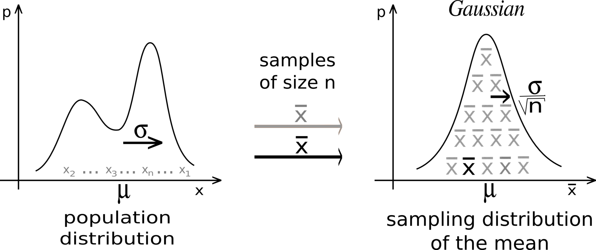
\(\overline{X} \sim N\!\Big(\mu, \dfrac{\sigma^2}{n}\Big)\)
The Central Limit Theorem says: Even if \(X\) is not normally distributed, for sufficiently large sample size \(n\), the distribution of the sample mean \(\overline{X}\) is approximately normal with:
\(\overline{X} \approx N\!\Big(\mu, \dfrac{\sigma^2}{n}\Big)\)
This approximation becomes more accurate as \(n\) increases. In practice, \(n \geq 30\) is often considered “large enough”.
This result is powerful because it allows us to use normal probability methods to make inferences about the mean, even if the population is not normal.
Example:
A factory produces nails. The length of a single nail has mean \(\mu = 5.0 \ \text{cm}\) and standard deviation \(\sigma = 0.2 \ \text{cm}\). The distribution of lengths is not normal but is slightly skewed. A sample of \(n = 64\) nails is taken. Find the approximate probability that the sample mean length is less than \(4.95 \ \text{cm}\).
▶️ Answer/Explanation
Step 1: By the CLT, for \(n=64\), \(\overline{X}\) is approximately normal:
\(\overline{X} \sim N\!\Big(5.0, \dfrac{0.2^2}{64}\Big) = N(5.0, 0.000625)\)
So, \(\text{SE} = \sqrt{0.000625} = 0.025\).
Step 2: Standardize:
\(P(\overline{X} < 4.95) = P\!\left(Z < \dfrac{4.95 – 5.0}{0.025}\right)\)
= \(P(Z < -2)\)
Step 3: From Normal tables: \(P(Z < -2) = 0.0228\).
Thus, the probability is \(\boxed{0.0228}\).
Example:
The weight of apples in a market has mean \(\mu = 150 \ \text{g}\) and standard deviation \(\sigma = 30 \ \text{g}\). The distribution is not normal (it is skewed). A sample of \(n = 100\) apples is chosen. Find the probability that the sample mean weight lies between \(145 \ \text{g}\) and \(155 \ \text{g}\).
▶️ Answer/Explanation
Step 1: By CLT, \(\overline{X}\) is approximately normal:
\(\overline{X} \sim N\!\Big(150, \dfrac{30^2}{100}\Big) = N(150, 9)\)
So, \(\text{SE} = 3\).
Step 2: Standardize bounds:
\(P(145 < \overline{X} < 155) = P\!\left(\dfrac{145-150}{3} < Z < \dfrac{155-150}{3}\right)\)
= \(P(-1.67 < Z < 1.67)\)
Step 3: From Normal tables:
\(P(Z < 1.67) = 0.9525, \quad P(Z < -1.67) = 0.0475\)
So, probability = \(0.9525 – 0.0475 = 0.905\).
Thus, the probability is \(\boxed{0.905}\).
Unbiased Estimates of Mean and Variance
When we take a sample from a population, we usually want to estimate the population mean \(\mu\) and variance \(\sigma^2\).
The word unbiased means that, although any one sample may give an estimate that is too high or too low, the process of sampling gives the correct value on average.
Sample Mean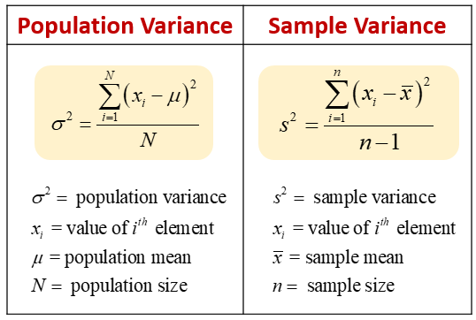
The sample mean is:
\(\overline{x} = \dfrac{1}{n}\sum_{i=1}^n x_i\)
This is an unbiased estimator of the population mean \(\mu\), because \(E(\overline{X}) = \mu\).
Sample Variance
To estimate the population variance, we do not use the “naïve” formula \(\dfrac{1}{n}\sum (x_i – \overline{x})^2\), because that tends to underestimate \(\sigma^2\).
Instead, we use:
\(s^2 = \dfrac{1}{n-1} \sum_{i=1}^n (x_i – \overline{x})^2\)
This is the unbiased estimator of \(\sigma^2\). The denominator is \(n-1\) (not \(n\)).
Using Summarised Data
If we are given totals instead of raw data, we can use these formulas:
\(\overline{x} = \dfrac{\sum x}{n}\)
\(s^2 = \dfrac{1}{n-1}\left(\sum x^2 – \dfrac{(\sum x)^2}{n}\right)\)
Example:
A sample of 5 observations is: 4, 6, 5, 7, 8. Find unbiased estimates of the population mean and variance.
▶️ Answer/Explanation
Step 1: Sample mean:
\(\overline{x} = \dfrac{4+6+5+7+8}{5} = \dfrac{30}{5} = 6\)
Step 2: Deviations from mean and squares:
\((4-6)^2 = 4, \ (6-6)^2 = 0, \ (5-6)^2 = 1, \ (7-6)^2 = 1, \ (8-6)^2 = 4\)
\(\sum (x_i – \overline{x})^2 = 10\)
Step 3: Sample variance:
\(s^2 = \dfrac{10}{5-1} = \dfrac{10}{4} = 2.5\)
So, \(\boxed{\mu \approx 6, \ \sigma^2 \approx 2.5}\)
Example:
A sample of size \(n=6\) has \(\sum x = 36\) and \(\sum x^2 = 232\). Find unbiased estimates of the population mean and variance.
▶️ Answer/Explanation
Step 1: Sample mean:
\(\overline{x} = \dfrac{\sum x}{n} = \dfrac{36}{6} = 6\)
Step 2: Sample variance formula:
\(s^2 = \dfrac{1}{n-1}\Big(\sum x^2 – \dfrac{(\sum x)^2}{n}\Big)\)
= \(\dfrac{1}{5}\Big(232 – \dfrac{36^2}{6}\Big)\)
= \(\dfrac{1}{5}\Big(232 – 216\Big) = \dfrac{16}{5} = 3.2\)
So, \(\boxed{\mu \approx 6, \ \sigma^2 \approx 3.2}\)
Confidence Interval for a Population Mean
A confidence interval (CI) gives a range of values within which the population mean \(\mu\) is likely to lie, based on the sample mean \(\overline{X}\).The confidence level (e.g. 95%) represents the long-run proportion of confidence intervals that would contain the true mean if we repeated the sampling many times.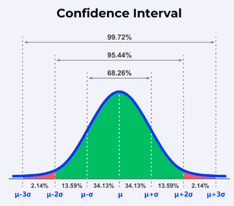
Formula for Confidence Interval:
- If the population variance \(\sigma^2\) is known and the sample mean comes from a normal distribution (or large \(n\)), then:
\(\overline{X} \pm z_{\alpha/2} \dfrac{\sigma}{\sqrt{n}}\)
- Here, \(z_{\alpha/2}\) is the critical value from the standard normal distribution (e.g. 1.96 for 95% confidence).
Interpretation:
- A 95% confidence interval means: “We are 95% confident that the population mean \(\mu\) lies within this interval.”
- It does not mean there is a 95% probability that \(\mu\) lies inside the interval (since \(\mu\) is fixed).
Example:
A machine produces screws. A sample of \(n = 100\) screws has a mean length \(\overline{X} = 5.02 \, \text{cm}\). The population standard deviation is known: \(\sigma = 0.1 \, \text{cm}\). Find a 95% confidence interval for the true mean length.
▶️ Answer/Explanation
Step 1: Write the formula:
CI = \(\overline{X} \pm z_{0.025} \dfrac{\sigma}{\sqrt{n}}\)
Step 2: Substituting values:
\(\overline{X} = 5.02, \; \sigma = 0.1, \; n = 100, \; z_{0.025} = 1.96\)
Margin of error = \(1.96 \times \dfrac{0.1}{\sqrt{100}} = 1.96 \times 0.01 = 0.0196\)
Step 3: Construct the interval:
\(5.02 \pm 0.0196 \Rightarrow (5.0004, 5.0396)\)
Final Answer:
\(\boxed{(5.0004 \, \text{cm}, \; 5.0396 \, \text{cm})}\)
We are 95% confident that the true mean screw length lies between 5.0004 cm and 5.0396 cm
Confidence Interval for a Population Proportion
When we want to estimate the true proportion \(p\) of a population that has a certain characteristic, we often use a sample proportion \(\hat{p}\). From a large sample, we can build a confidence interval for \(p\).
The sample proportion is given by: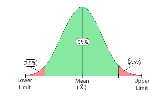
\(\hat{p} = \dfrac{x}{n}\)
where \(x\) is the number of successes and \(n\) is the sample size.
For large \(n\), by the Central Limit Theorem, \(\hat{p}\) is approximately normally distributed with:
Mean \(E(\hat{p}) = p\)
Variance \(\text{Var}(\hat{p}) = \dfrac{p(1-p)}{n}\)
Since \(p\) is unknown, we estimate the standard error (SE) using \(\hat{p}\):
\(SE = \sqrt{\dfrac{\hat{p}(1-\hat{p})}{n}}\)
A confidence interval (CI) for the true population proportion is then:
\(\hat{p} \ \pm \ z \times SE\)
where \(z\) is the standard normal critical value (e.g. \(z = 1.96\) for 95% confidence).
Example:
A survey of 500 people finds that 320 support a new law. Find a 95% confidence interval for the true proportion of the population that supports the law.
▶️ Answer/Explanation
Step 1: Calculate sample proportion:
\(\hat{p} = \dfrac{320}{500} = 0.64\)
Step 2: Find standard error:
\(SE = \sqrt{\dfrac{0.64(1-0.64)}{500}} = \sqrt{\dfrac{0.2304}{500}} \approx 0.0215\)
Step 3: 95% confidence interval uses \(z = 1.96\):
Margin of error = \(1.96 \times 0.0215 \approx 0.0421\)
Step 4: Construct the interval:
\(0.64 \pm 0.0421 \implies (0.598, \ 0.682)\)
Final Answer:
\(\boxed{0.598 \leq p \leq 0.682}\)
We are 95% confident that the true proportion of the population who support the law is between 59.8% and 68.2%.