Understanding Hypothesis Testing
A hypothesis test is a formal procedure for testing a claim (hypothesis) about a population parameter using sample data.
- Null Hypothesis (\(H_0\)): The default assumption or claim. Usually states that there is no effect or no difference.
- Alternative Hypothesis (\(H_1\) or \(H_a\)): The competing claim, usually stating that there is an effect or difference.
- Significance Level (\(\alpha\)): The probability threshold for rejecting \(H_0\). Common values: \(0.05\), \(0.01\).
- Test Statistic: A value calculated from the sample data that is compared against a distribution (e.g., standard normal) to make a decision.
- Critical Region (or Rejection Region): Range of values for the test statistic where \(H_0\) is rejected.
- Acceptance Region: Range of values where \(H_0\) is not rejected.
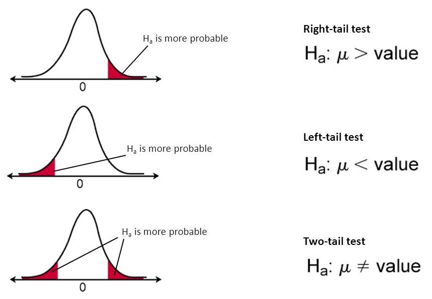
One-tailed vs Two-tailed Tests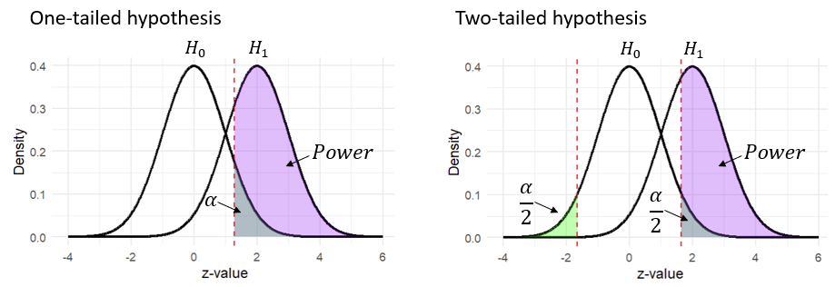
One-tailed test: Tests for an effect in only one direction.
Example: \(H_0: \mu = 50\), \(H_1: \mu > 50\)
Two-tailed test: Tests for an effect in both directions.
Example: \(H_0: \mu = 50\), \(H_1: \mu \neq 50\)
Example:
A company claims the mean lifetime of its light bulbs is \(1000 \, \text{hours}\). A sample of \(n=36\) bulbs has a mean of \(\overline{x} = 980\) hours. Assume population standard deviation \(\sigma = 60\). Test at the \(5\%\) significance level whether the claim is valid.
▶️ Answer/Explanation
Step 1: State hypotheses
\(H_0: \mu = 1000\)
\(H_1: \mu \neq 1000\) (two-tailed)
Step 2: Compute test statistic
Standard error: \(SE = \dfrac{\sigma}{\sqrt{n}} = \dfrac{60}{\sqrt{36}} = 10\)
\(Z = \dfrac{\overline{x} – \mu}{SE} = \dfrac{980 – 1000}{10} = -2.0\)
Step 3: Determine critical region
At \(\alpha = 0.05\), two-tailed test → critical values: \(\pm 1.96\).
Step 4: Decision
Since \(-2.0 < -1.96\), test statistic lies in the rejection region.
Final Answer:
Reject \(H_0\). There is sufficient evidence at the \(5\%\) level to say the mean lifetime is different from \(1000 \, \text{hours}\).
Hypothesis Testing with Binomial and Poisson Distributions
Steps in Hypothesis Testing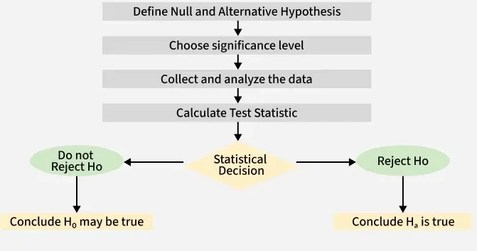
- State the null hypothesis \(H_0\): assumes no effect or no difference (status quo).
- State the alternative hypothesis \(H_1\): represents what we are testing for (change or effect).
- Select a significance level \(\alpha\) (commonly 0.05 or 0.01).
- Identify the test statistic (depends on the distribution: binomial, Poisson, or normal approximation).
- Find the rejection (critical) region based on the distribution and \(\alpha\).
- Compare the observed data with the rejection region → reject or fail to reject \(H_0\).
Hypothesis Tests with the Binomial Distribution
If \(X \sim \text{Bin}(n, p)\), then under \(H_0\), the probability of \(x\) successes is:
\(P(X = x) = \binom{n}{x} p^x (1-p)^{n-x}\)
Critical regions are found by summing probabilities in the tail(s) depending on one- or two-tailed tests.
Example:
A factory claims that 90% of its bulbs last more than 1000 hours. A sample of \(n=20\) bulbs shows only 15 last longer than 1000 hours. Test the claim at the 5% level.
▶️ Answer/Explanation
Step 1: Hypotheses
\(H_0: p = 0.9\), \(H_1: p < 0.9\) (one-tailed test).
Step 2: Test Statistic
\(X \sim \text{Bin}(20, 0.9)\). Observed value: \(x=15\).
Step 3: Rejection Region
Find \(P(X \leq 15)\) under \(H_0\).
Step 4: Calculation
Using binomial probabilities: \(P(X \leq 15) = \sum_{k=0}^{15} \binom{20}{k} (0.9)^k (0.1)^{20-k}\). This gives approximately \(0.041\).
Step 5: Conclusion
Since \(0.041 < 0.05\), we reject \(H_0\). There is evidence that fewer than 90% of bulbs last more than 1000 hours.
Hypothesis Tests with the Poisson Distribution
If \(X \sim \text{Po}(\lambda)\), then under \(H_0\), the probability of \(x\) events is:
\(P(X = x) = \dfrac{e^{-\lambda} \lambda^x}{x!}\)
Critical regions are formed by adding probabilities in one or both tails.
Example:
A call centre receives an average of 5 calls per minute. In a one-minute interval, 10 calls were received. Test whether the rate of calls has increased at the 5% level.
▶️ Answer/Explanation
Step 1: Hypotheses
\(H_0: \lambda = 5\), \(H_1: \lambda > 5\) (one-tailed test).
Step 2: Test Statistic
\(X \sim \text{Po}(5)\). Observed value: \(x=10\).
Step 3: Rejection Region
Find \(P(X \geq 10)\).
Step 4: Calculation
\(P(X \geq 10) = 1 – P(X \leq 9)\). Using Poisson probabilities, \(P(X \geq 10) \approx 0.0318\).
Step 5: Conclusion
Since \(0.0318 < 0.05\), we reject \(H_0\). There is evidence that the call rate has increased.
Hypothesis Tests for the Population Mean
A hypothesis test is used to determine whether there is enough statistical evidence in a sample to infer that a population parameter (here, the mean) differs from a claimed value.
Steps of a Hypothesis Test for the Mean:
Step 1: State hypotheses
Null hypothesis: \(H_0: \mu = \mu_0\)
Alternative hypothesis: \(H_1: \mu \neq \mu_0\), \(H_1: \mu > \mu_0\), or \(H_1: \mu < \mu_0\) depending on whether the test is two-tailed, right-tailed, or left-tailed.
Step 2: Test statistic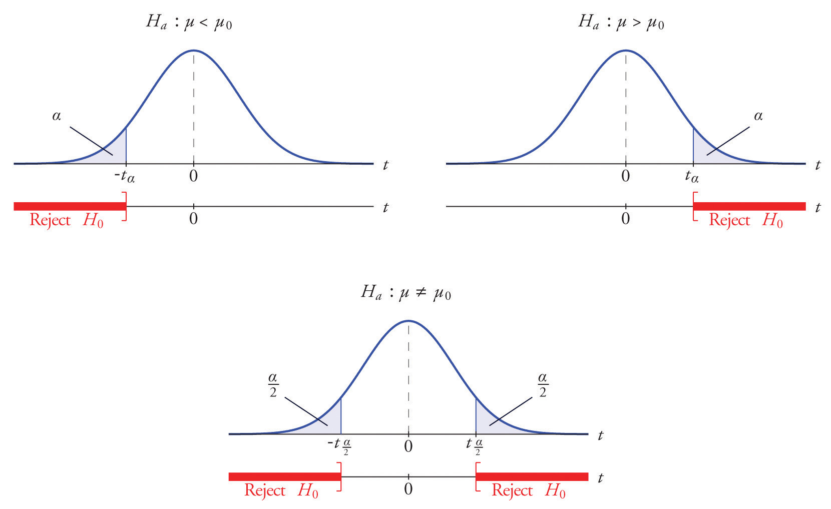
If population variance \(\sigma^2\) is known or \(n\) is large, the test statistic is:
\( Z = \dfrac{\overline{X} – \mu_0}{\sigma / \sqrt{n}} \)
This follows approximately a standard normal distribution under \(H_0\).
Step 3: Rejection region
Decide the significance level (\(\alpha\)), e.g. 5%.
For a two-tailed test: reject \(H_0\) if \(|Z| > z_{\alpha/2}\).
For a one-tailed test: reject \(H_0\) if \(Z > z_\alpha\) (right-tailed) or \(Z < -z_\alpha\) (left-tailed).
Step 4: Conclusion
Compare test statistic to critical value. State conclusion in context.
Example:
A machine fills cereal packets. The target mean weight is \(500 \, \text{g}\). A sample of \(n = 36\) packets has a mean weight of \(495 \, \text{g}\). It is known that the population standard deviation is \(\sigma = 12 \, \text{g}\). Test at the 5% significance level whether the machine is filling packets correctly.
▶️ Answer/Explanation
Step 1: Hypotheses
\(H_0: \mu = 500\)
\(H_1: \mu \neq 500\) (two-tailed test)
Step 2: Test statistic
\(Z = \dfrac{\overline{X} – \mu_0}{\sigma / \sqrt{n}} = \dfrac{495 – 500}{12 / \sqrt{36}} = \dfrac{-5}{2} = -2.5\)
Step 3: Rejection region
For 5% significance (two-tailed): reject \(H_0\) if \(|Z| > 1.96\).
Step 4: Conclusion
Here \(|Z| = 2.5 > 1.96\), so we reject \(H_0\).
There is significant evidence at the 5% level that the mean packet weight is not \(500 \, \text{g}\).
Final Answer: \(\boxed{\text{The machine is not filling packets correctly.}}\)
Type I and Type II Errors
When performing a hypothesis test, we make a decision based on sample evidence. Since samples are subject to chance variation, there is always the possibility of making an incorrect conclusion. These incorrect decisions are classified as Type I error and Type II error.
Type I Error: Rejecting the null hypothesis \(H_0\) when it is actually true.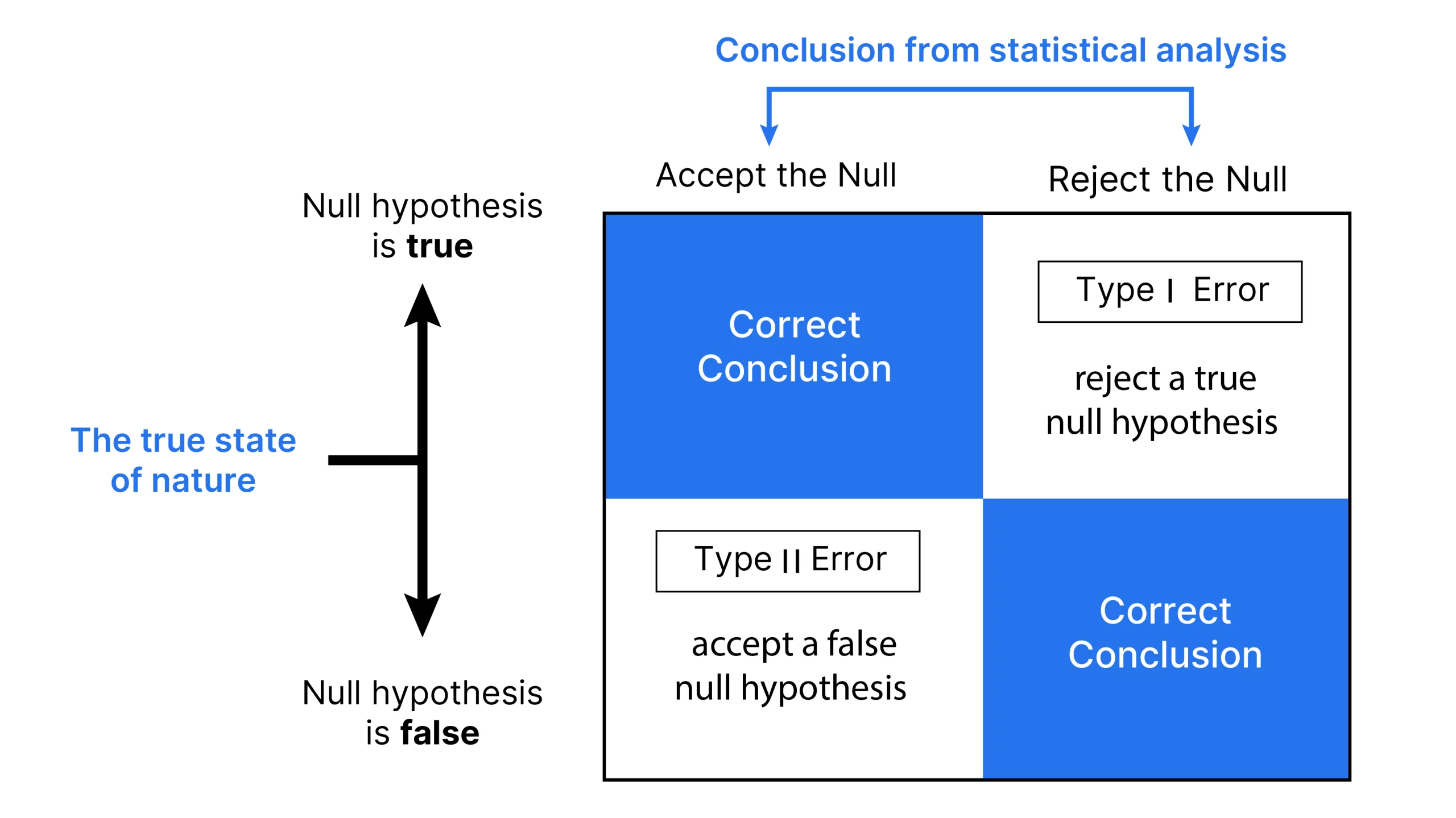
This is a “false positive”.
The probability of making a Type I error is the significance level of the test, usually denoted by \(\alpha\).
Type II Error: Failing to reject the null hypothesis \(H_0\) when the alternative hypothesis \(H_1\) is actually true.
This is a “false negative”.
The probability of making a Type II error is denoted by \(\beta\).
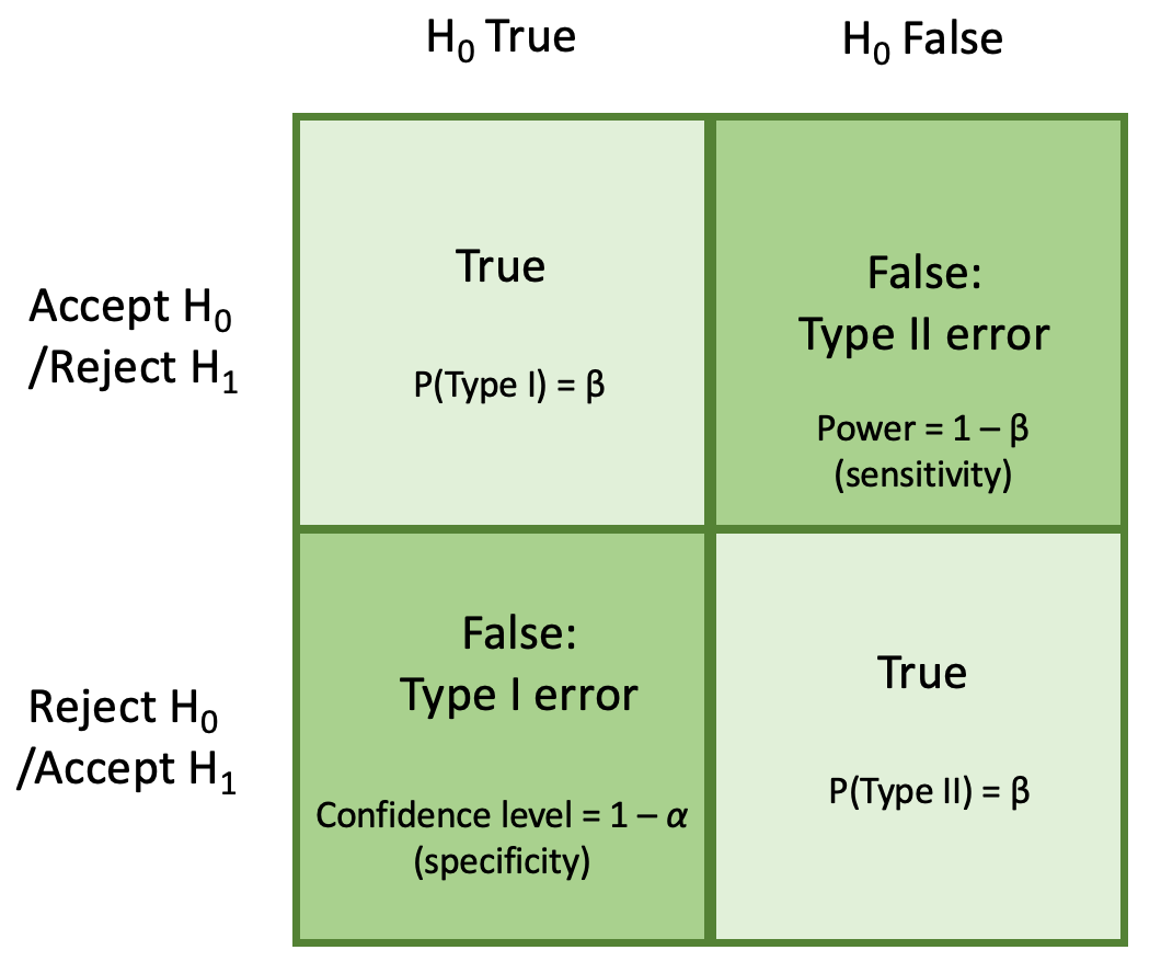
Power of a Test
- The power of a test is defined as \(1 – \beta\).
It represents the probability of correctly rejecting \(H_0\) when \(H_1\) is true.
Example:
A company claims that the mean weight of their product is \(500 \, \text{g}\). A consumer protection group suspects that the mean weight is actually less than \(500 \, \text{g}\). They test this with a hypothesis test at 5% significance level.
- \(H_0: \mu = 500\)
- \(H_1: \mu < 500\)
▶️ Explanation of Errors
Type I Error: The test concludes the mean is less than 500 g (rejects \(H_0\)) when in fact the mean is exactly 500 g. This means accusing the company unfairly.
Type II Error: The test concludes there is no evidence the mean is less than 500 g (fails to reject \(H_0\)) when in fact the mean is less than 500 g. This means failing to detect underweight products.
Power: The probability of correctly detecting underweight products when they truly exist.
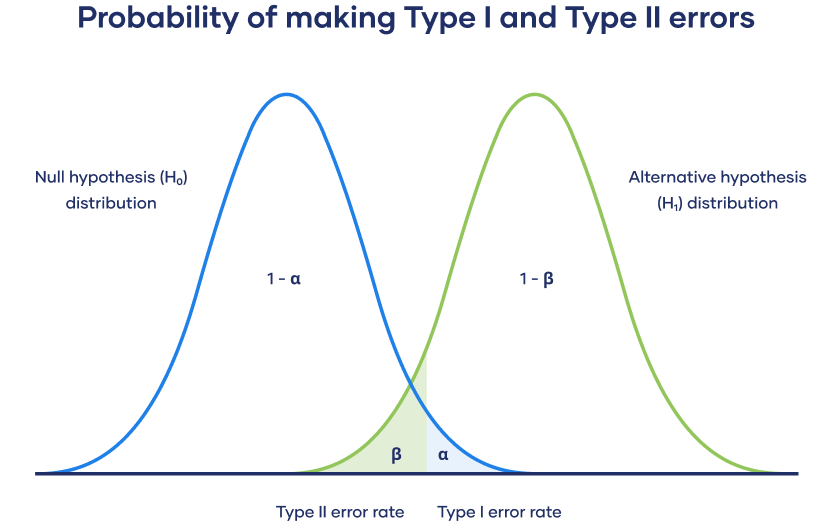
How to find Type I and Type II error probabilities
Type I error (α): probability of rejecting \(H_0\) when \(H_0\) is true. This is determined by the chosen rejection region and the distribution under \(H_0\).
Type II error (β): probability of failing to reject \(H_0\) when a specified alternative is true. To compute β you evaluate the probability that the test statistic falls in the acceptance region, but under the distribution specified by the alternative hypothesis.
Procedure:
(1) State \(H_0\) and \(H_1\).
(2) Choose α and find the rejection region under \(H_0\).
(3) Compute α (sanity check).
(4) Compute β by evaluating the acceptance-region probability under the alternative.
Example — Normal (known variance)
Test \(H_0:\mu=100\) vs \(H_1:\mu>100\). Population standard deviation \(\sigma=10\). Sample size \(n=25\). Use \(\alpha=0.05\) (one-tailed).
▶️ Answer / Explanation
Step A — critical value and rejection region (under \(H_0\))
For one-tailed \(\alpha=0.05\), \(z_{0.05}=1.645\).
Critical value for \(\overline{X}\): \(\overline{x}_c = \mu_0 + z_{0.05}\dfrac{\sigma}{\sqrt{n}} = 100 + 1.645\cdot\dfrac{10}{\sqrt{25}}\).
Compute \(\dfrac{10}{\sqrt{25}} = \dfrac{10}{5} = 2\). So \(\overline{x}_c = 100 + 1.645\times 2 = 100 + 3.29 = 103.29.\)
Rejection region: \(\overline{X} > 103.29\). By design \(\alpha = 0.05\).
Step B — Type II error β for a specific alternative, say \(\mu=105\)
We need \(\beta = P\big(\overline{X} \le 103.29 \mid \mu=105\big)\).
Standardize: \(Z = \dfrac{\overline{X}-\mu}{\sigma/\sqrt{n}}\). So
\(\beta = P\!\left(Z \le \dfrac{103.29-105}{2}\right) = P\!\left(Z \le \dfrac{-1.71}{2}\right) = P(Z \le -0.855)\).
From standard normal tables \(P(Z \le -0.855) \approx 0.196\).
Results:
\(\boxed{\alpha = 0.05,\quad \beta \approx 0.196,\quad \text{power }=1-\beta\approx 0.804}\).
Example — Binomial (direct evaluation)
Test \(H_0: p=0.5\) vs \(H_1:p>0.5\). Sample size \(n=10\). Reject \(H_0\) if \(X\ge 8\) (number of successes).
▶️ Answer / Explanation
Step A — Type I error α (under \(p=0.5\))
\(\alpha = P(X\ge 8 \mid p=0.5) = P(X=8)+P(X=9)+P(X=10)\).
For \(n=10,\; p=0.5\):
\(P(X=8)=\dfrac{\binom{10}{8}}{2^{10}}=\dfrac{45}{1024}\approx 0.0439453.\)
\(P(X=9)=\dfrac{10}{1024}\approx 0.0097656,\quad P(X=10)=\dfrac{1}{1024}\approx 0.0009766.\)
So \(\alpha \approx 0.0439453+0.0097656+0.0009766 = 0.0546875.\)
Step B — Type II error β for alternative \(p=0.7\)
\(\beta = P(\text{fail to reject}) = P(X\le 7 \mid p=0.7) = 1 – P(X\ge 8 \mid p=0.7)\).
Compute \(P(X\ge 8)\) under \(p=0.7\):
Using \(n=10\):
\(P(X=8)=45\cdot 0.7^8\cdot0.3^2 \approx 0.23347444.\)
\(P(X=9)=10\cdot 0.7^9\cdot0.3 \approx 0.12106082.\)
\(P(X=10)=0.7^{10}\approx 0.02824852.\)
So \(P(X\ge8)\approx 0.23347444+0.12106082+0.02824852 = 0.38278378.\)
Thus \(\beta \approx 1 – 0.38278378 = 0.61721622.\)
Results:
\(\boxed{\alpha \approx 0.05469,\quad \beta \approx 0.61722,\quad \text{power}\approx 0.38278}\).
Example — Poisson (direct evaluation)
Test \(H_0:\lambda=3\) vs \(H_1:\lambda>3\). A single observation \(X\sim\text{Po}(\lambda)\). Reject \(H_0\) if \(X\ge 7\).
▶️ Answer / Explanation
Step A — Type I error α (under \(\lambda=3\))
\(\alpha = P(X\ge 7\mid \lambda=3) = 1 – P(X\le 6\mid \lambda=3)\).
Compute \(P(X=k)=e^{-3}\dfrac{3^k}{k!}\). Summing \(k=0\) to \(6\) gives \(P(X\le 6)\approx 0.96649144\).
So \(\alpha \approx 1 – 0.96649144 = 0.03350856.\)
Step B — Type II error β for alternative \(\lambda=5\)
\(\beta = P(\text{fail to reject}) = P(X\le 6 \mid \lambda=5)\).
Compute \(P(X\le 6)\) for \(\lambda=5\) by summing \(k=0\) to \(6\): this gives approximately \(0.76218346\).
So \(\beta \approx 0.76218346\) and power \(\approx 0.23781654\).
Results:
\(\boxed{\alpha \approx 0.03351,\quad \beta \approx 0.76218,\quad \text{power}\approx 0.23782}\).