CIE AS/A level Probability & Statistics 2 Paper 6 Prediction - 2025
CIE AS/A level Probability & Statistics 2 Paper 6 Prediction- 2025
To excel in A level Math Exam, consistent practice with CIE AS & A Level Revision resources is key. CIE AS/A level Probability & Statistics 2 Paper 6 Prediction will guide you for exam pattern.
IITian Academy offers a vast collection of questions that can aid your understanding of specific topics and solidify your concepts. By practicing regularly and focusing on these key areas, you’ll be well-prepared for the A level Math exam
Question 1
A random sample of 250 people living in Barapet was chosen. It was found that 78 of these people owned a BETEC phone.
(a) Calculate an approximate 98% confidence interval for the proportion of people living in Barapet who own a BETEC phone.
(b) Manjit claims that more than 40% of the people living in Barapet own a BETEC phone. Use your answer to part (a) to comment on this claim.
▶️Answer/Explanation
Solution: –
Let’s solve this concisely, focusing on clarity and precision.
(a) Calculate an approximate 98% confidence interval for the proportion of people living in Barapet who own a BETEC phone
Given:
– Sample size \(n = 250\)
– Number of people owning a BETEC phone = 78
– Sample proportion \( \hat{p} = \frac{78}{250} = 0.312 \)
We use the formula for the confidence interval for a proportion:
\[ \hat{p} \pm Z \cdot \sqrt{\frac{\hat{p}(1 – \hat{p})}{n}} \]
For a 98% confidence level, the Z-score (from standard normal distribution) is approximately 2.326 (since \(P(Z < 2.326) \approx 0.99\), so \(P(-2.326 < Z < 2.326) = 0.98\)).
Calculate the standard error (SE):
\[ \hat{p}(1 – \hat{p}) = 0.312 \cdot (1 – 0.312) = 0.312 \cdot 0.688 = 0.214656 \]
\[ \frac{\hat{p}(1 – \hat{p})}{n} = \frac{0.214656}{250} \approx 0.000858624 \]
\[ \sqrt{0.000858624} \approx 0.0293 \]
Now, the margin of error (ME):
\[ ME = 2.326 \cdot 0.0293 \approx 0.0681 \]
So, the 98% confidence interval is:
\[ 0.312 – 0.0681 \text{ to } 0.312 + 0.0681 \]
\[ 0.2439 \text{ to } 0.3801 \]
Thus, the approximate 98% confidence interval is:
\[ (0.244, 0.380) \]
(b) Comment on Manjit’s claim that more than 40% of the people living in Barapet own a BETEC phone
Manjit claims \(p > 0.40\) (where \(p\) is the true proportion of people in Barapet owning a BETEC phone).
– The upper bound of the 98% confidence interval is 0.380 (or 38.0%).
– Since 0.40 (40%) is greater than 0.380, it lies outside the confidence interval.
This suggests that, at the 98% confidence level, we do not have sufficient evidence to support Manjit’s claim that more than 40% of people in Barapet own a BETEC phone. The data indicates the true proportion is likely less than 40%.
Final Answers
(a) Approximate 98% confidence interval: (0.244, 0.380)
(b) Manjit’s claim that more than 40% of people in Barapet own a BETEC phone is not supported by the confidence interval, as 0.40 lies outside the interval (0.244, 0.380).
——————Markscheme———–
2(a) $\frac{78}{250} \pm z \times \sqrt{\frac{\frac{78}{250}\times(1-\frac{78}{250})}{250}}$
$z = 2.326$
= 0.244 to 0.38[0] (3 sf)
2(b) Unlikely to be true because confidence interval does not contain 0.4.
Question 2
Each year a transport firm uses $X$ litres of gasoline and $Y$ litres of diesel fuel, where $X$ and $Y$ have the independent distributions $X \sim N(10700, 950^{2})$ and $Y \sim N(13400, 1210^{2})$.
(a) Find the probability that in a randomly chosen year the firm uses more gasoline than diesel fuel.
The costs per litre of gasoline and diesel fuel are $0.80 and $0.85 respectively.
(b) Find the probability that the total cost of gasoline and diesel fuel in a randomly chosen year is between $20 000 and $22 000.
▶️Answer/Explanation
Solution: –
Let’s solve this concisely, focusing on clarity and precision.
(a) Find the probability that in a randomly chosen year the firm uses more gasoline than diesel fuel
Given:
\(X \sim N(10700, 950^2)\), so \(\mu_X = 10700\), \(\sigma_X = 950\).
\(Y \sim N(13400, 1210^2)\), so \(\mu_Y = 13400\), \(\sigma_Y = 1210\).
We need \(P(X > Y)\).
Since \(X\) and \(Y\) are independent, \(X – Y \sim N(\mu_X – \mu_Y, \sigma_X^2 + \sigma_Y^2)\):
\(\mu_{X – Y} = 10700 – 13400 = -2700\)
\(\sigma_{X – Y}^2 = 950^2 + 1210^2 = 902500 + 1464100 = 2366600\)
\(\sigma_{X – Y} = \sqrt{2366600} \approx 1538.3\)
We need \(P(X – Y > 0)\):
\[ Z = \frac{0 – (-2700)}{1538.3} = \frac{2700}{1538.3} \approx 1.755 \]
Using the standard normal distribution, \(P(Z > 1.755) = 1 – P(Z \leq 1.755)\):
– \(P(Z \leq 1.755) \approx 0.960\) (from standard normal tables).
– \(P(Z > 1.755) \approx 1 – 0.960 = 0.040\)
So, the probability is approximately:
\[ \text{Probability} \approx 0.040 \]
(b) Find the probability that the total cost of gasoline and diesel fuel in a randomly chosen year is between $20,000 and $22,000
Cost of gasoline = \(0.80 \cdot X\), where \(X \sim N(10700, 950^2)\).
Cost of diesel = \(0.85 \cdot Y\), where \(Y \sim N(13400, 1210^2)\).
Total cost \(T = 0.80X + 0.85Y\).
Since \(X\) and \(Y\) are independent, \(T\) is normally distributed:
\(\mu_T = 0.80 \cdot 10700 + 0.85 \cdot 13400\)
\[ 0.80 \cdot 10700 = 8560 \]
\[ 0.85 \cdot 13400 = 11390 \]
\[ \mu_T = 8560 + 11390 = 19950 \]
\(\sigma_T^2 = (0.80)^2 \cdot 950^2 + (0.85)^2 \cdot 1210^2\)
\[ 0.80^2 = 0.64, \quad 950^2 = 902500, \quad 0.64 \cdot 902500 = 577600 \]
\[ 0.85^2 = 0.7225, \quad 1210^2 = 1464100, \quad 0.7225 \cdot 1464100 = 1058262.5 \]
\[ \sigma_T^2 = 577600 + 1058262.5 = 1635862.5 \]
\(\sigma_T = \sqrt{1635862.5} \approx 1278.8\)
We need \(P(20000 < T < 22000)\):
\[ Z_1 = \frac{20000 – 19950}{1278.8} = \frac{50}{1278.8} \approx 0.0391 \]
\[ Z_2 = \frac{22000 – 19950}{1278.8} = \frac{2050}{1278.8} \approx 1.603 \]
Using the standard normal distribution:
\(P(Z \leq 0.0391) \approx 0.516\) (from standard normal tables).
\(P(Z \leq 1.603) \approx 0.946\).
\[ P(0.0391 < Z < 1.603) = 0.946 – 0.516 = 0.430 \]
So, the probability is approximately:
\[ \text{Probability} \approx 0.430 \]
Final Answers
(a) 0.040
(b) 0.430
—————-Marscheme—————-
4(a) E(X-Y) = 10700 – 13400 [-=2700]
Var(X-Y) = 950^{2} + 1210^{2} [=2366600]
$\frac{0-(\text{their ‘}-2700’)}{\sqrt{\text{their ‘2366600’}}} [=1.755]$
$1-\Phi(\text{their ‘1.755’})$
= 0.0396 or 0.0397 (3 sf)
4(b) E(Total) = 10700 \times 0.8 + 13400 \times 0.85 [=19950]
Var(Total) = 950^{2} \times 0.8^{2} + 1210^{2} \times 0.85^{2} [=1635412.25]
$\frac{22000-\text{their ‘19950’}}{\sqrt{\text{their ‘1635412.25’}}} [=1.603] \text{ or } \frac{20000-\text{their ‘19950’}}{\text{their ‘1635412.25’}} [=0.0391]$
$\Phi(\text{their ‘1.603’})-\Phi(\text{their ‘0.0391’}) = 0.9455-0.5156$
= 0.43[0] (3 sf)
Question 3
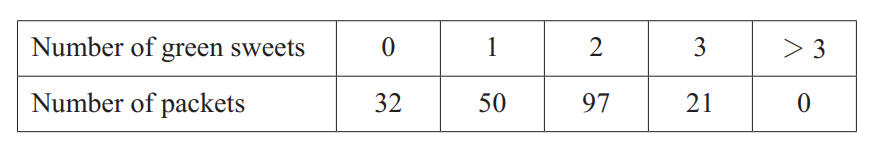
The numbers of green sweets in 200 randomly chosen packets of Frutos are summarised in the table.
(a) Calculate an unbiased estimate for the population mean of the number of green sweets in a packet of Frutos, and show that an unbiased estimate of the population variance is $0.783$ correct to 3 significant figures.
The manufacturers of Frutos claim that the mean number of green sweets in a packet is 1.65.
Anji believes that the true value of the mean, $\mu$, is less than 1.65. She uses the results from the 200 randomly chosen packets to test the manufacturers’ claim.
(b) State suitable null and alternative hypotheses for the test.
(c) Show that the result of Anji’s test is significant at the 5% level but not at the 1% level.
(d) It is given that Anji made a Type I error.
Explain how this shows that the significance level that Anji used in her test was not 1%.
▶️Answer/Explanation
Solution: –
(a) Calculate unbiased estimates of the mean and variance, and show variance = 0.783 (3 s.f.).
Data: 200 packets, frequencies: 0 (32), 1 (50), 2 (97), 3 (21), >3 (0).
Total packets = 32 + 50 + 97 + 21 = 200.
Mean (\(\bar{x}\)):
\[
\bar{x} = \frac{\sum x \cdot f}{\sum f} = \frac{0 \cdot 32 + 1 \cdot 50 + 2 \cdot 97 + 3 \cdot 21}{200} = \frac{0 + 50 + 194 + 63}{200} = \frac{307}{200} = 1.535
\]
Unbiased estimate of population mean: 1.535.
**Variance (\(s^2\))** (unbiased, using \(n-1\)):
\[
s^2 = \frac{\sum (x – \bar{x})^2 \cdot f}{n-1} = \frac{\sum x^2 \cdot f – \frac{(\sum x \cdot f)^2}{n}}{n-1}
\]
\[
\sum x \cdot f = 307, \quad (\sum x \cdot f)^2 = 307^2 = 94249
\]
\[
\sum x^2 \cdot f = 0^2 \cdot 32 + 1^2 \cdot 50 + 2^2 \cdot 97 + 3^2 \cdot 21 = 0 + 50 + 388 + 189 = 627
\]
\[
\frac{(\sum x \cdot f)^2}{n} = \frac{94249}{200} = 471.245
\]
\[
\sum x^2 \cdot f – \frac{(\sum x \cdot f)^2}{n} = 627 – 471.245 = 155.755
\]
\[
s^2 = \frac{155.755}{199} \approx 0.7826 \approx 0.783 \quad (\text{to 3 s.f.})
\]
Unbiased estimate of variance: 0.783.
(b) State suitable null and alternative hypotheses.
\(H_0: \mu = 1.65\), \(H_1: \mu < 1.65\) (one-tailed test, testing if mean is less than 1.65).
(c) Show the test is significant at 5% but not at 1%.
Test statistic (z-score):
\[
z = \frac{\bar{x} – \mu_0}{\sigma / \sqrt{n}}, \quad \sigma = \sqrt{0.783} \approx 0.8849, \quad n = 200
\]
\[
z = \frac{1.535 – 1.65}{0.8849 / \sqrt{200}} = \frac{-0.115}{0.8849 / 14.142} = \frac{-0.115}{0.0626} \approx -1.837
\]
– For 5% significance (one-tailed), critical \(z = -1.645\).
Since \(-1.837 < -1.645\), reject \(H_0\) at 5% (significant).
– For 1% significance, critical \(z = -2.326\).
Since \(-1.837 > -2.326\), do not reject \(H_0\) at 1% (not significant).
(d) Explain how a Type I error shows the significance level was not 1%.
A Type I error occurs if \(H_0\) is rejected when true (\(\mu = 1.65\)).
Given Anji made a Type I error, she rejected \(H_0\) at her chosen significance level \(\alpha\), but the test was not significant at 1% (\(z = -1.837 > -2.326\)).
If \(\alpha = 1\%\), she would not reject \(H_0\) (since \(z > -2.326\)), so a Type I error at 1% is impossible.
Thus, \(\alpha\) must be greater than 1%, and since the test is significant at 5% but not 1%, Anji likely used \(\alpha = 5\%\).
——————-Markscheme————-
6(a) $\hat{\mu}=\frac{307}{200}$ or 1.535
$\Sigma x^{2}f=627, \text{Est}(\sigma^2) = \frac{200(627)-1.535^{2}}{199}$ or $\frac{1}{199}(627 -\frac{307^{2}}{200})$
$= 0.783$
6(b) $H_0: \mu=1.65$
$H_1: \mu<1.65$
6(c) $\frac{1.535-1.65}{\sqrt{0.783\div200}}$
= -1.838 or -1.84
$\Phi(0.05)$ and $\Phi(0.01)$ attempted
-1.645 > -1.838 > -2.326
Hence significant at 5% but not 1% level
6(d) At the 1% level $H_{0}$ is not rejected
Or a Type I error can only occur if $H_{0}$ is rejected.
Question 4
A random variable X has probability density function f given by
\[f(x)=\begin{cases}
ax-x^{3} & 0 \leq x \leq \sqrt{2}, \\
0 & \text{otherwise,}
\end{cases}\]
where a is a constant.
(a) Show that $a = 2$.
(b) Find the median of $X$.
(c) Find the exact value of $E(X)$
▶️Answer/Explanation
Solution: –
(a) Show that \(a = 2\).
The total area under \(f(x)\) must equal 1:
\[
\int_0^{\sqrt{2}} (ax – x^3) \, dx = 1
\]
\[
\left[ \frac{ax^2}{2} – \frac{x^4}{4} \right]_0^{\sqrt{2}} = \frac{a(\sqrt{2})^2}{2} – \frac{(\sqrt{2})^4}{4} = \frac{2a}{2} – \frac{4}{4} = a – 1
\]
\[
a – 1 = 1, \quad a = 2
\]
Thus, \(a = 2\), so \(f(x) = 2x – x^3\), \(0 \leq x \leq \sqrt{2}\).
(b) Find the median of \(X\).
Median \(m\) satisfies \(P(X \leq m) = 0.5\):
\[
\int_0^m (2x – x^3) \, dx = 0.5
\]
\[
\left[ x^2 – \frac{x^4}{4} \right]_0^m = m^2 – \frac{m^4}{4} = 0.5
\]
\[
4m^2 – m^4 = 2
\]
\[
m^4 – 4m^2 + 2 = 0
\]
Let \(u = m^2\), so:
\[
u^2 – 4u + 2 = 0
\]
\[
u = \frac{4 \pm \sqrt{16 – 8}}{2} = \frac{4 \pm \sqrt{8}}{2} = \frac{4 \pm 2\sqrt{2}}{2} = 2 \pm \sqrt{2}
\]
\[
u = 2 + \sqrt{2} \approx 3.414, \quad u = 2 – \sqrt{2} \approx 0.586
\]
Since \(0 \leq m \leq \sqrt{2} \approx 1.414\), \(m^2 \leq 2\):
– \(u = 2 – \sqrt{2} \approx 0.586\) (valid, \(m = \sqrt{0.586} \approx 0.765\)).
– \(u = 2 + \sqrt{2} > 2\), invalid.
Check \(m \approx 0.765\):
\[
\int_0^{0.765} (2x – x^3) \, dx = [x^2 – \frac{x^4}{4}]_0^{0.765} = (0.765)^2 – \frac{(0.765)^4}{4}
\]
\[
0.765^2 \approx 0.585, \quad 0.765^4 \approx 0.343, \quad \frac{0.343}{4} \approx 0.0858
\]
\[
0.585 – 0.0858 = 0.4992 \approx 0.5
\]
Median: 0.765 (approximately, exact \(\sqrt{2 – \sqrt{2}}\)).
(c) Find the exact value of \(E(X)\).
\[
E(X) = \int_0^{\sqrt{2}} x (2x – x^3) \, dx = \int_0^{\sqrt{2}} (2x^2 – x^4) \, dx
\]
\[
\left[ \frac{2x^3}{3} – \frac{x^5}{5} \right]_0^{\sqrt{2}} = \frac{2(\sqrt{2})^3}{3} – \frac{(\sqrt{2})^5}{5}
\]
\[
(\sqrt{2})^3 = 2\sqrt{2}, \quad (\sqrt{2})^5 = 4\sqrt{2}
\]
\[
\frac{2 \cdot 2\sqrt{2}}{3} – \frac{4\sqrt{2}}{5} = \frac{4\sqrt{2}}{3} – \frac{4\sqrt{2}}{5} = 4\sqrt{2} \left( \frac{1}{3} – \frac{1}{5} \right) = 4\sqrt{2} \cdot \frac{5 – 3}{15} = 4\sqrt{2} \cdot \frac{2}{15} = \frac{8\sqrt{2}}{15}
\]
Exact value of \(E(X)\): \(\frac{8\sqrt{2}}{15}\).
———Markscheme————–
5(a) $\int_{0}^{\sqrt{2}}(ax-x^{3})dx=1$
$\left[a\frac{x^{2}}{2}-\frac{x^{4}}{4}\right]_{0}^{\sqrt{2}}=1$
$a-\frac{4}{4}=1$
$a=2$
5(b) $\int_{0}^{m}(2x-x^{3})dx=\frac{1}{2}$
$m^{2}-\frac{m^{4}}{4}=\frac{1}{2}$
$m^{4}-4m^{2}+2=0 \Rightarrow m^{2}=\frac{4\pm\sqrt{16-8}}{2}$
$m= 2 \pm \sqrt{2}$
$m=\sqrt{2-\sqrt{2}}$ or 0.765 (3sf)
5(c) $\int_{0}^{\sqrt{2}}(2x^{2}-x^{4})dx$
$\left[\frac{2x^{3}}{3}-\frac{x^{5}}{5}\right]_{0}^{\sqrt{2}}$
$\left[=\frac{4\sqrt{2}}{3}-\frac{4\sqrt{2}}{5}\right] = \frac{8}{15}\sqrt{2}$
Question 5
The heights, in centimetres, of adult females in Litania have mean $\mu$ and standard deviation $\sigma$. It is known that in 2004 the values of $\mu$ and $\sigma$ were 163.21 and 6.95 respectively. The government claims that the value of $\mu$ this year is greater than it was in 2004. In order to test this claim a researcher plans to carry out a hypothesis test at the 1% significance level. He records the heights of a random sample of 300 adult females in Litania this year and finds the value of the sample mean.
(a) State the probability of a Type I error.
You should assume that the value of $\sigma$ after 2004 remains at 6.95.
(b) Given that the value of $\mu$ this year is actually 164.91, find the probability of a Type II error.
▶️Answer/Explanation
Solution: –
Solution:
We define the hypotheses for the hypothesis test:
- Null hypothesis:
- Alternative hypothesis:
(since we are testing if the mean height has increased)
The sample size is
, and the population standard deviation remains
.
(a) Probability of a Type I Error
A Type I error occurs when we reject
even though it is true. Since the test is conducted at the 1% significance level, the probability of a Type I error is simply:
Thus, the answer is:
(b) Probability of a Type II Error
A Type II error occurs when we fail to reject
even though the true mean has increased to
.
Step 1: Find the Critical Value
The sample mean follows a normal distribution:
The standard error:
At the 1% significance level (right-tailed test), the critical value
corresponding to
is:
The critical sample mean value is:
Thus, we reject
if
.
Step 2: Compute Probability of Type II Error
If the true mean is
, then:
We need to find:
Standardizing:
From normal tables:
Thus, the probability of a Type II error is:
—————Markscheme—————-
(a) 0.01 or 1\%
(b) $2.326 = \frac{\overline{h}-163.21}{\frac{6.95}{\sqrt{300}}}$
$\overline{h} = 164.14$
[Rejection region is $\overline{h} > 164.14$]
[P(Type II) = P($\overline{h}<164.14|\mu=164.91$)]
$\frac{\text{their ‘164.14’-164.91}}{\frac{6.95}{\sqrt{300}}} = -1.919$
$\Phi(\text{their ‘}-1.919’) = 1 – \Phi(\text{their ‘1.919’}) = 0.0275 \text{ or } 0.0276 \text{ or } 0.028[0] \text{ (3 s.f)}$
Question 6
A teacher models the numbers of girls and boys who arrive late for her class on any day by the independent random variables $G \sim Po(0.10)$ and $B \sim Po(0.15)$ respectively.
(a) Find the probability that during a randomly chosen 2-day period no girls arrive late.
(b) Find the probability that during a randomly chosen 5-day period the total number of students who arrive late is less than 3.
(c) It is given that the values of $P(G=r)$ and $P(B=r)$ for $r \geq 3$ are very small and can be ignored.
Find the probability that on a randomly chosen day more girls arrive late than boys.
Following a timetable change the teacher claims that on average more students arrive late than before the change. During a randomly chosen 5-day period a total of 4 students are late.
(d) Test the teacher’s claim at the 5% significance level.
▶️Answer/Explanation
Solution: –
(a) Find the probability that during a randomly chosen 2-day period no girls arrive late
– \(G \sim Po(0.10)\), the number of girls arriving late per day.
– For a 2-day period, the total number of girls arriving late \(G_{\text{total}} \sim Po(2 \cdot 0.10) = Po(0.20)\).
– We need \(P(G_{\text{total}} = 0)\):
\[ P(G_{\text{total}} = 0) = e^{-0.20} \approx 0.8187 \]
So, the probability is approximately:
\[ \text{Probability} \approx 0.819 \]
(b) Find the probability that during a randomly chosen 5-day period the total number of students who arrive late is less than 3
\(G \sim Po(0.10)\), \(B \sim Po(0.15)\), and \(G\) and \(B\) are independent.
– For a 5-day period, the total number of girls late \(G_{\text{total}} \sim Po(5 \cdot 0.10) = Po(0.50)\).
– The total number of boys late \(B_{\text{total}} \sim Po(5 \cdot 0.15) = Po(0.75)\).
– Total students late \(T = G_{\text{total}} + B_{\text{total}}\). Since \(G_{\text{total}}\) and \(B_{\text{total}}\) are independent Poisson variables, \(T \sim Po(0.50 + 0.75) = Po(1.25)\).
– We need \(P(T < 3) = P(T = 0) + P(T = 1) + P(T = 2)\):
\[ P(T = k) = \frac{\lambda^k e^{-\lambda}}{k!}, \quad \lambda = 1.25 \]
\(P(T = 0) = e^{-1.25} \approx 0.2865\)
\(P(T = 1) = 1.25 e^{-1.25} \approx 1.25 \cdot 0.2865 = 0.3581\)
\(P(T = 2) = \frac{1.25^2 e^{-1.25}}{2} = \frac{1.5625 \cdot 0.2865}{2} \approx \frac{0.4475}{2} = 0.2238\)
\[ P(T < 3) \approx 0.2865 + 0.3581 + 0.2238 = 0.8684 \]
So, the probability is approximately:
\[ \text{Probability} \approx 0.868 \]
(c) Find the probability that on a randomly chosen day more girls arrive late than boys, given \(P(G = r)\) and \(P(B = r)\) for \(r \geq 3\) are very small and can be ignored
– \(G \sim Po(0.10)\), \(B \sim Po(0.15)\), and \(G\) and \(B\) are independent.
– We need \(P(G > B)\), ignoring \(G \geq 3\) and \(B \geq 3\) (since their probabilities are very small).
– Possible values for \(G\) and \(B\) are 0, 1, or 2 (since \(P(G \geq 3)\) and \(P(B \geq 3)\) are negligible).
Calculate probabilities:
\(P(G = 0) = e^{-0.10} \approx 0.9048\)
\(P(G = 1) = 0.10 e^{-0.10} \approx 0.10 \cdot 0.9048 = 0.0905\)
\(P(G = 2) = \frac{0.10^2 e^{-0.10}}{2} = \frac{0.01 \cdot 0.9048}{2} \approx \frac{0.009048}{2} = 0.0045\)
\(P(B = 0) = e^{-0.15} \approx 0.8607\)
\(P(B = 1) = 0.15 e^{-0.15} \approx 0.15 \cdot 0.8607 = 0.1291\)
\(P(B = 2) = \frac{0.15^2 e^{-0.15}}{2} = \frac{0.0225 \cdot 0.8607}{2} \approx \frac{0.01936}{2} = 0.0097\)
Now, find \(P(G > B)\):
\(G = 0\): \(B\) must be 0 for \(G > B\), but \(P(G = 0, B = 0) = 0.9048 \cdot 0.8607 \approx 0.7786\). Since \(0 \not> 0\), this contributes 0.
\(G = 1\): \(B = 0\) (since \(1 > 0\), but \(1 \not> 1\) or \(1 \not> 2\)).
\[ P(G = 1, B = 0) = 0.0905 \cdot 0.8607 \approx 0.0779 \]
\(G = 2\): \(B = 0\) or \(B = 1\) (since \(2 > 0\), \(2 > 1\), but \(2 \not> 2\)).
\[ P(G = 2, B = 0) = 0.0045 \cdot 0.8607 \approx 0.0039 \]
\[ P(G = 2, B = 1) = 0.0045 \cdot 0.1291 \approx 0.0006 \]
\[ P(G = 2, B = 0 \text{ or } 1) \approx 0.0039 + 0.0006 = 0.0045 \]
\[ P(G > B) \approx 0.0779 + 0.0045 = 0.0824 \]
So, the probability is approximately:
\[ \text{Probability} \approx 0.082 \]
(d) Test the teacher’s claim that on average more students arrive late than before the change, given a total of 4 students are late over a 5-day period, at the 5% significance level
Before the change, total students late per day \(T = G + B \sim Po(0.10 + 0.15) = Po(0.25)\).
Teacher claims \(\lambda > 0.25\) (more students late on average).
For 5 days, \(T_{\text{total}} \sim Po(5 \cdot 0.25) = Po(1.25)\).
Observed \(T_{\text{total}} = 4\). Test \(H_0: \lambda = 1.25\) vs. \(H_1: \lambda > 1.25\) at 5% significance.
Use a Poisson test. The critical value for a one-tailed test at 5% significance for \(Po(1.25)\) is the smallest \(k\) where \(P(X \geq k) \leq 0.05\):
\(P(X \geq 3) = 1 – P(X < 3) = 1 – 0.8684 \approx 0.1316\) (from part (b)).
\(P(X \geq 4) = 1 – [P(X = 0) + P(X = 1) + P(X = 2) + P(X = 3)]\):
\(P(X = 3) = \frac{1.25^3 e^{-1.25}}{6} = \frac{1.953125 \cdot 0.2865}{6} \approx \frac{0.5595}{6} \approx 0.0933\)
\(P(X < 4) \approx 0.2865 + 0.3581 + 0.2238 + 0.0933 = 0.9617\)
\(P(X \geq 4) = 1 – 0.9617 = 0.0383\)
Since \(P(X \geq 4) = 0.0383 < 0.05\), the critical value is 4. If \(X \geq 4\), reject \(H_0\).
– Observed \(X = 4\), which is the critical value. At the 5% level, we reject \(H_0\) because \(P(X \geq 4) = 0.0383 < 0.05\).
Thus, there is sufficient evidence at the 5% significance level to support the teacher’s claim that more students arrive late than before the change.
Final Answers
(a) 0.819
(b) 0.868
(c) 0.082
(d) Reject \(H_0\) at the 5% significance level; there is sufficient evidence to support the teacher’s claim that more students arrive late than before the change.
——————-Markscheme——————
(a) $[e^{-0.2}] = 0.819 (3 sf)$
(b) $\lambda = 1.25$
$e^{-1.25}\left(1+1.25+\frac{1.25^{2}}{2}\right)$
or $e^{-1.25}(1+1.25+0.78125)$
or $0.2865 + 0.3581 + 0.2238$
= $0.868 (3 sf)$
(c)
$e^{-0.15} \times e^{0.1} \times (0.1) = 0.077879$
$e^{-0.15} \times e^{0.1} \times \frac{(0.1)^2}{2} = 0.003894$
$e^{-0.15} \times 0.15 \times e^{0.1} \times \frac{(0.1)^2}{2} = 0.0005841$
$e^{-0.15} \times e^{0.1} \times (0.1) + e^{-0.15} \times e^{0.1} \times \frac{(0.1)^2}{2} + e^{-0.15} \times 0.15 \times e^{0.1} \times \frac{(0.1)^2}{2} = 0.077879 + 0.003894 + 0.0005841 = 0.0824 \text{ (3 sf)}$
Alternative method for Question 5(c)
$P(B=0) \times P(G>0) = e^{-0.15} \times (1-e^{-0.1})$
$P(B=1) \times P(G>1) = e^{-0.15} \times 0.15 \times (1-e^{-0.1}(1+0.1))$
$e^{-0.15} \times (1-e^{-0.1}) + e^{-0.15} \times 0.15 \times (1-e^{-0.1}(1+0.1)) = 0.0824 \text{ (3 sf)}$
(d)
$H_0: \lambda = 1.25 \text{ or } 0.25 \text{[per day]}$
$H_1: \lambda > 1.25 \text{ or } 0.25 \text{[per day]}$
$P(\text{4 or fewer late}) = 1 – e^{-1.25}(1+1.25+\frac{1.25^2}{2!}+\frac{1.25^3}{3!})$
$= 1 – e^{-1.25}(1+1.25+0.7813+0.3255)$
$= 1 – (0.2865 + 0.3581 + 0.2238 + 0.09326)$
$= 0.0383$
$0.0383 < 0.05$
$\therefore$ Reject $H_0$
Hence there is sufficient evidence to suggest that the teacher’s claim is true.
or
There is sufficient evidence to suggest that more students are late on average.
Question 7
Every July, as part of a research project, Rita collects data about sightings of a particular kind of bird.
Each day in July she notes whether she sees this kind of bird or not, and she records the number X of days on which she sees it. She models the distribution of X by B(31, p), where p is the probability of seeing this kind of bird on a randomly chosen day in July.
Data from previous years suggests that p = 0.3, but in 2022 Rita suspected that the value of p had been reduced. She decided to carry out a hypothesis test.
In July 2022, she saw this kind of bird on 4 days.
(a) Use the binomial distribution to test at the 5% significance level whether Rita’s suspicion is justified.
In July 2023, she noted the value of X and carried out another test at the 5% significance level using the same hypotheses.
(b) Calculate the probability of a Type I error.
Rita models the number of sightings, Y, per year of a different, very rare, kind of bird by the distribution B(365, 0.01).
(c) (i) Use a suitable approximating distribution to find P(Y=4).
(ii) Justify your approximating distribution in this context.
▶️Answer/Explanation
Solution: –
7(a) $H_0: p=0.3$
$H_1: p<0.3$
$P(X\le4) =$
\[0.7^{31}+31\times0.7^{30}\times0.3+{}^{31}C_{2}\times0.7^{29}\times0.3^{2}+{}^{31}C_{3}\times0.7^{28}\times0.3^{3}+^{31}C_{4}\times 0.7^{24}\times 0.3^{4}\]
\[= 0.00001577 + 0.0002096 + 0.0013475 + 0.0055826 + 0.016748\]
$$= 0.0239 (3sf)$$
‘There is sufficient evidence (at 5% level) to support Rita’s
suspicion’, or ‘There is sufficient evidence to suggest the probability of seeing
this type of bird has decreased’
7(b) $P(X\le5) = [0.0239 + ^{31}C_{5}\times0.7^{26}\times0.3^{5}] = 0.0627$ [which is > 0.05]
7(c) (i) $[\lambda=] 3.65$
$e^{-3.65} \times \frac{3.65^{4}}{4!}$
= 0.192 (3sf)
7(c) (ii) $n = 365 > 50$
$np = 3.65 < 5$ or $p = 0.01 < 0.1$