Calculus and Limits for Understanding Dynamic Change
Calculus is the mathematics of change. It allows us to model and analyze how quantities vary in relation to each other. The foundation of calculus is the concept of a limit, which describes the value that a function approaches as the input approaches some point.
Dynamic change in calculus:
The average rate of change of a function \( f(x) \) over an interval
\([a, b]\) is: \( \frac{f(b) – f(a)}{b – a} \)
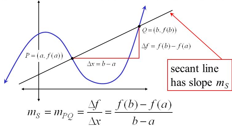
This gives the slope of the secant line connecting two points on the curve.
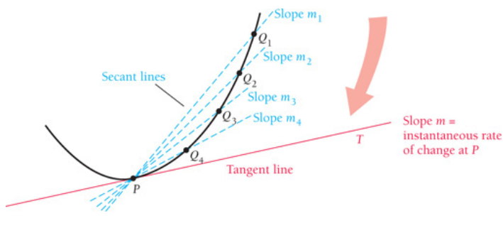
The instantaneous rate of change at a point \( x = a \) is the limit of average rates as the interval becomes infinitely small:
\( f'(a) = \lim_{h \to 0} \frac{f(a + h) – f(a)}{h} \)
This gives the slope of the tangent line at that point.
Similarly, the definite integral is defined using limits to add up infinitely many small areas under a curve:
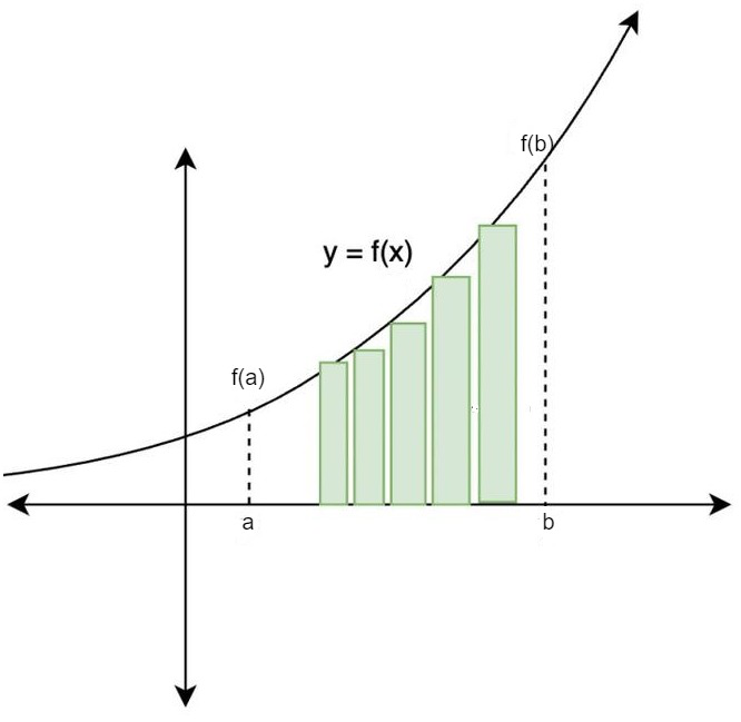
\( \int_a^b f(x) \, dx \)
This models accumulated change (such as total distance, area, or quantity).
The limit process connects average quantities over intervals with exact values at specific points, enabling precise modeling of dynamic systems.
Average Rate of Change

The average rate of change of a function \( f(x) \) between two points \( x = a \) and \( x = b \) is the change in \( y \)-value divided by the change in \( x \)-value:
\( \text{Average rate of change} = \frac{f(b) – f(a)}{b – a} \)
It represents the slope of the secant line connecting \( (a, f(a)) \) and \( (b, f(b)) \) on the graph of \( f(x) \).
In real contexts, this could describe the average speed over a time interval, or average growth rate over a domain.
Example:
Find the average rate of change of \( f(x) = x^2 + 2x \) between \( x = 1 \) and \( x = 4 \).
▶️ Answer/Explanation
Compute \( f(4) \)
\( f(4) = 4^2 + 2 \cdot 4 = 16 + 8 = 24 \}
Compute \( f(1) \)
\( f(1) = 1^2 + 2 \cdot 1 = 1 + 2 = 3 \}
Compute average rate of change
\( \frac{f(4) – f(1)}{4 – 1} = \frac{24 – 3}{3} = \frac{21}{3} = 7 \}
Example:
A particle moves along a straight line, and its position at time \( t \) is given by \( s(t) = t^3 – 6t^2 + 9t \), where \( s \) is in meters and \( t \) is in seconds.
Find the average velocity of the particle between \( t = 1 \) and \( t = 4 \).
▶️ Answer/Explanation
Compute \( s(4) \)
\( s(4) = (4)^3 – 6(4)^2 + 9(4) = 64 – 96 + 36 = 4 \)
Compute \( s(1) \)
\( s(1) = (1)^3 – 6(1)^2 + 9(1) = 1 – 6 + 9 = 4 \)
Compute average velocity
\( \text{Average velocity} = \frac{s(4) – s(1)}{4 – 1} = \frac{4 – 4}{3} = 0 \)
Final answer:
The average velocity between \( t = 1 \) and \( t = 4 \) is: \( 0 \ \text{m/s} \)
The particle ends up at the same position at \( t = 4 \) as it was at \( t = 1 \), so the average velocity is zero.
Limits and Instantaneous Rate of Change
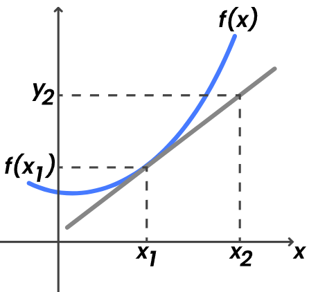
The instantaneous rate of change of a function at a point is the slope of the tangent line at that point.
We approximate this by looking at the average rate of change over a small interval:
\( \frac{f(x + h) – f(x)}{h} \) where \( h \) is the difference between the two x-values.
The instantaneous rate of change is defined as:
\( \lim_{h \to 0} \frac{f(x + h) – f(x)}{h} \)
The limit bridges the gap between average rate of change over an interval and the exact rate of change at a point.
Example:
Find the instantaneous rate of change of \( f(x) = x^2 \) at \( x = 2 \) using the limit definition.
▶️ Answer/Explanation
Write the average rate of change expression
\( \frac{f(2 + h) – f(2)}{h} = \frac{(2 + h)^2 – 2^2}{h} \)
Simplify the numerator
\( = \frac{(4 + 4h + h^2) – 4}{h} = \frac{4h + h^2}{h} \) \( = 4 + h \)
Take the limit as \( h \to 0 \)
\( \lim_{h \to 0} (4 + h) = 4 \)
Final answer:
The instantaneous rate of change at \( x = 2 \) is: \( 4 \)
Example:
Find the instantaneous rate of change of \( f(x) = 3x^2 + 2x \) at \( x = 2 \) using the limit definition.
▶️ Answer/Explanation
Write the limit definition at \( x = 2 \)
\( f'(2) = \lim_{h \to 0} \frac{f(2 + h) – f(2)}{h} \)
Compute \( f(2 + h) \) and \( f(2) \)
\( f(2 + h) = 3(2 + h)^2 + 2(2 + h) = 3(4 + 4h + h^2) + 4 + 2h = 12 + 12h + 3h^2 + 4 + 2h = 16 + 14h + 3h^2 \)
\( f(2) = 3(2)^2 + 2(2) = 3(4) + 4 = 12 + 4 = 16 \)
Form the difference quotient
\( = \lim_{h \to 0} \frac{16 + 14h + 3h^2 – 16}{h} = \lim_{h \to 0} \frac{14h + 3h^2}{h} \)
\( = \lim_{h \to 0} (14 + 3h) = 14 \)