Finding Taylor Polynomial Approximations of Functions
A Taylor polynomial is a polynomial that approximates a function near a specific point \( a \). The idea is to match the function’s value and as many derivatives as possible at \( x = a \). As the degree of the polynomial increases, the approximation becomes more accurate near \( a \).
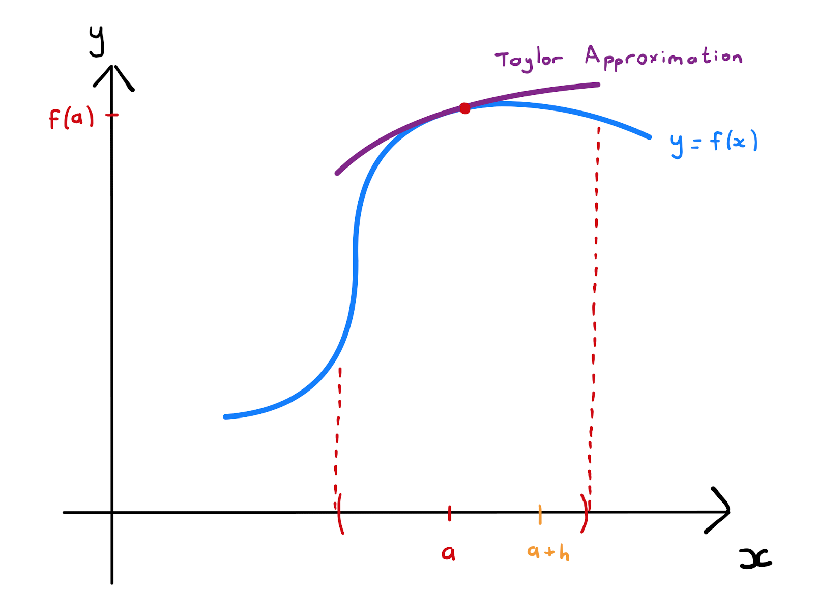
The nth-degree Taylor polynomial for a function \( f(x) \) centered at \( x = a \) is:
\( \displaystyle P_n(x) = f(a) + f'(a)(x-a) + \dfrac{f”(a)}{2!}(x-a)^2 + \dfrac{f^{(3)}(a)}{3!}(x-a)^3 + \dots + \dfrac{f^{(n)}(a)}{n!}(x-a)^n \)
If \( a = 0 \), the polynomial is called a Maclaurin polynomial.
Purpose:
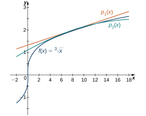
In many cases, as the degree of a Taylor polynomial increases, the \( n \)th-degree polynomial will approach the original function over some interval around the center \( a \). This means that for large \( n \), \( P_n(x) \) can be made arbitrarily close to \( f(x) \) within that interval, provided that \( f \) is sufficiently smooth (infinitely differentiable) there.
This is why Taylor polynomials are a powerful tool for approximations higher-degree polynomials capture more curvature and local behavior of the function, making the approximation accurate over a wider range of \( x \).
- Approximate complicated functions using polynomials for easier computation.
- Estimate function values that are difficult to compute directly.
- Analyze local behavior of functions near a given point.
Steps to Find a Taylor Polynomial Approximation:
- Choose the center \( a \) and degree \( n \).
- Compute \( f(a) \), \( f'(a) \), \( f”(a) \), …, \( f^{(n)}(a) \).
- Substitute these values into the Taylor polynomial formula.
- Simplify to get \( P_n(x) \).
- Use \( P_n(x) \) to approximate \( f(x) \) near \( a \).
Error Term (Taylor’s Remainder):
The difference between \( f(x) \) and \( P_n(x) \) is the remainder term:
\( \displaystyle R_n(x) = \dfrac{f^{(n+1)}(c)}{(n+1)!}(x-a)^{n+1} \) where \( c \) is between \( a \) and \( x \).
This term estimates the error in the approximation.
Example
Find the 3rd-degree Maclaurin polynomial for \( f(x) = e^x \).
▶️ Answer/Explanation
Compute derivatives at \( x = 0 \):
\( f(x) = e^x \), \( f'(x) = e^x \), \( f”(x) = e^x \), \( f^{(3)}(x) = e^x \) At \( x = 0 \): \( f(0) = 1 \), \( f'(0) = 1 \), \( f”(0) = 1 \), \( f^{(3)}(0) = 1 \)
Apply formula:
\( P_3(x) = 1 + x + \dfrac{x^2}{2!} + \dfrac{x^3}{3!} = 1 + x + \dfrac{x^2}{2} + \dfrac{x^3}{6} \)
Conclusion: This polynomial approximates \( e^x \) near \( x = 0 \).
Example
Find the 2nd-degree Taylor polynomial for \( f(x) = \ln(x) \) centered at \( a = 1 \).
▶️ Answer/Explanation
Compute derivatives at \( x = 1 \):
\( f(x) = \ln(x) \) → \( f'(x) = \dfrac{1}{x} \), \( f”(x) = -\dfrac{1}{x^2} \) At \( x = 1 \): \( f(1) = 0 \), \( f'(1) = 1 \), \( f”(1) = -1 \)
Apply formula:
\( P_2(x) = 0 + 1(x – 1) + \dfrac{-1}{2}(x – 1)^2 \) \( P_2(x) = (x – 1) – \dfrac{(x – 1)^2}{2} \)
Conclusion: This polynomial approximates \( \ln(x) \) near \( x = 1 \).
Example
The function \( f \) has derivatives of all orders for all real \( x \), with \( f(0) = 0 \), \( f'(0) = 2 \), \( f”(0) = -3 \), \( f^{(3)}(0) = 4 \). Write the 3rd-degree Maclaurin polynomial for \( f \).
▶️ Answer/Explanation
Apply Maclaurin formula:
\( P_3(x) = f(0) + f'(0)x + \dfrac{f”(0)}{2!}x^2 + \dfrac{f^{(3)}(0)}{3!}x^3 \)
Substitute:
\( P_3(x) = 0 + 2x + \dfrac{-3}{2}x^2 + \dfrac{4}{6}x^3 \) \( P_3(x) = 2x – \dfrac{3}{2}x^2 + \dfrac{2}{3}x^3 \)
Conclusion: This polynomial approximates \( f(x) \) near \( x = 0 \).