Rates of Change in Applied Contexts Other Than Motion
The concept of a derivative as a rate of change is widely used outside of physical motion.In real-world applications, derivatives can describe how quantities vary in fields such as economics, biology, medicine, engineering, and environmental science.
In general: If \( y = f(x) \), then the derivative \( f'(x) \) gives the rate of change of \( y \) with respect to \( x \). The units of the derivative are “units of \( y \)” per “unit of \( x \)”.
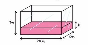
Example : How much time it will take to fill up completely
Key Ideas:
- Economics: Marginal cost, marginal revenue, and marginal profit are all derivatives of cost, revenue, and profit functions.
- Biology: Derivatives can describe how populations grow or shrink over time.
- Medicine: Drug concentration levels in the bloodstream change over time and can be studied using derivatives.
- Engineering: Rates of thermal change or mechanical stress are captured using derivatives.
- Environmental Science: Derivatives can model how pollution levels change in ecosystems.
Example:
The cost function of a company is given by \( C(x) = 5x^2 + 20x + 100 \), where \( x \) is the number of units produced.
Find the marginal cost when \( x = 10 \).
▶️Answer/Explanation
Marginal cost is the derivative of the cost function:
\( C'(x) = 10x + 20 \)
At \( x = 10 \),
\( C'(10) = 10(10) + 20 = 120 \)
So, the marginal cost is 120 units per item at 10 units.
Example:
The population of a bacteria culture is modeled by \( P(t) = 100e^{0.3t} \), where \( t \) is time in hours.
Find the rate of change of the population at \( t = 5 \).
▶️Answer/Explanation
\( P'(t) = 100 \cdot 0.3e^{0.3t} = 30e^{0.3t} \)
\( P'(5) = 30e^{1.5} \approx 30 \cdot 4.4817 \approx 134.45 \)
So, the population is growing at approximately 134.45 organisms per hour at \( t = 5 \).
Example:
A drug concentration in the blood is modeled by \( C(t) = \dfrac{50}{t + 1} \), where \( C(t) \) is the concentration in mg/L and \( t \) is time in hours.
Find the rate of change of the drug concentration at \( t = 2 \).
▶️Answer/Explanation
\( C'(t) = -\dfrac{50}{(t+1)^2} \)
\( C'(2) = -\dfrac{50}{(2+1)^2} = -\dfrac{50}{9} \approx -5.56 \)
The concentration is decreasing at a rate of about 5.56 mg/L per hour at \( t = 2 \).
Example:
The temperature of a heated object in degrees Celsius is given by \( T(t) = 80 – 20e^{-0.2t} \), where \( t \) is in minutes.
Find the rate of change of temperature at \( t = 3 \).
▶️Answer/Explanation
\( T'(t) = 20 \cdot 0.2e^{-0.2t} = 4e^{-0.2t} \)
\( T'(3) = 4e^{-0.6} \approx 4 \cdot 0.5488 \approx 2.195 \)
So, the temperature is increasing at about 2.20°C per minute at \( t = 3 \).
Example:
The pollution level in a lake is modeled by \( P(t) = 200 – 40\ln(t+1) \), where \( t \) is in years.
Find the rate of change of pollution level at \( t = 4 \).
▶️Answer/Explanation
\( P'(t) = -\dfrac{40}{t+1} \)
\( P'(4) = -\dfrac{40}{5} = -8 \)
Pollution is decreasing at a rate of 8 units per year at year 4.