Definite Integrals and Accumulated Change
Definite integrals are used to calculate the accumulated change of a quantity over an interval. They can represent the net area under a curve or total accumulation when the rate of change is known.
Definite integrals can be estimated or evaluated using:
- Graphical representations
- Numerical tables
- Analytical expressions (formulas)
- Verbal (real-world) descriptions
Meaning of a Definite Integral:
If \( f(x) \) is a rate of change function (like velocity), then the definite integral from \( a \) to \( b \) gives:
\(\displaystyle \int_a^b f(x)\,dx = \text{Net accumulation of the quantity over } [a, b] \)
Units of a Definite Integral:
If \( f(x) \) has units of units per x-unit (e.g. meters/second), and \( x \) has units of x-units (e.g. seconds), then the definite integral has units of:
\( (\text{units}/\text{x-unit}) \cdot (\text{x-unit}) = \text{units} \)
Signed vs Total Accumulation:
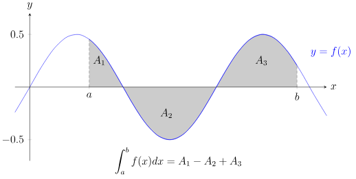
- Signed accumulation: Net value, considering positives and negatives (can cancel).
- Total accumulation: Sum of absolute values of areas (no canceling).
Example:
The table below gives values of a continuous function \( f(x) \), which represents a rate of change in gallons per hour. Approximate \(\displaystyle \int_0^4 f(x)\,dx \) using the trapezoidal rule.
| x (hours) | f(x) (gallons/hour) |
|---|---|
| 0 | 10 |
| 1 | 14 |
| 2 | 13 |
| 3 | 15 |
| 4 | 17 |
▶️Answer/Explanation
We use the trapezoidal rule for approximation:
\(\displaystyle \int_0^4 f(x)\,dx \approx \dfrac{1}{2}(10 + 14) + \dfrac{1}{2}(14 + 13) + \dfrac{1}{2}(13 + 15) + \dfrac{1}{2}(15 + 17) \)
\( = \dfrac{1}{2}(24) + \dfrac{1}{2}(27) + \dfrac{1}{2}(28) + \dfrac{1}{2}(32) = 12 + 13.5 + 14 + 16 = \boxed{55.5 \text{ gallons}} \)
This is the approximate accumulated amount of liquid added over 4 hours.
Approximating Definite Integrals Using Riemann and Trapezoidal Sums
When a function’s exact integral is difficult or impossible to compute analytically, we can approximate the definite integral using Riemann sums or the Trapezoidal Rule.
These approximations can be done using:
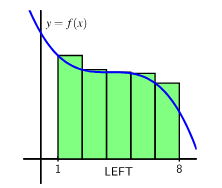
- Left Riemann Sum (LRS)
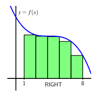
- Right Riemann Sum (RRS)
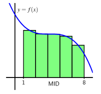
- Midpoint Riemann Sum (MRS)
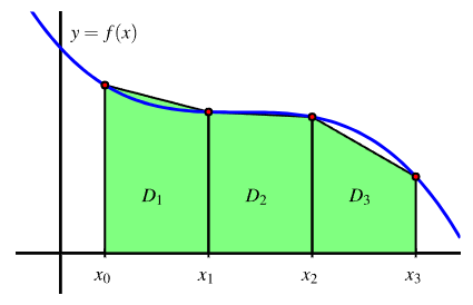
- Trapezoidal Sum (TRAP)
Uniform vs Nonuniform Partitions:
- Uniform partition: Subintervals have equal width.
- Nonuniform partition: Subintervals may have different widths.
Table of Approximation Methods
| Method | Expression | Uses Value at |
|---|---|---|
Left Riemann Sum | \( \sum f(x_i)\Delta x \) | Left endpoints |
Right Riemann Sum | \( \sum f(x_{i+1})\Delta x \) | Right endpoints |
Midpoint Riemann Sum | \( \sum f\left(\dfrac{x_i + x_{i+1}}{2}\right)\Delta x \) | Midpoints of subintervals |
Trapezoidal Rule | \( \sum \dfrac{f(x_i) + f(x_{i+1})}{2}\Delta x \) | Both endpoints of each interval |
Example:
The table shows values of a function \( f(x) \), which represents a car’s velocity in meters per second. Estimate the total distance traveled from \( x = 0 \) to \( x = 4 \) using:
- Left Riemann Sum
- Right Riemann Sum
- Midpoint Riemann Sum
- Trapezoidal Sum
| x (seconds) | f(x) (m/s) |
|---|---|
| 0 | 5 |
| 1 | 7 |
| 2 | 6 |
| 3 | 8 |
| 4 | 10 |
▶️Answer/Explanation
Subinterval width: \( \Delta x = 1 \)
- Left Riemann Sum: \( 1(5 + 7 + 6 + 8) = 26 \text{ meters} \)
- Right Riemann Sum: \( 1(7 + 6 + 8 + 10) = 31 \text{ meters} \)
- Midpoint Riemann Sum: Use values at \( x = 0.5, 1.5, 2.5, 3.5 \) → estimate using interpolation or graph
- Trapezoidal Rule:
\( \dfrac{1}{2}(5 + 7) + \dfrac{1}{2}(7 + 6) + \dfrac{1}{2}(6 + 8) + \dfrac{1}{2}(8 + 10) = 6 + 6.5 + 7 + 9 = \boxed{28.5 \text{ meters}} \)
Each estimate gives a sense of the total distance traveled from \( x = 0 \) to \( x = 4 \) seconds.
Numerical Approximation of Definite Integrals Using Technology
Technology can be used (e.g., a graphing calculator or software like Desmos, GeoGebra, or a CAS-enabled device) to approximate definite integrals using methods such as left, right, midpoint, or trapezoidal sums. The method chosen can affect whether the approximation is an underestimate or overestimate depending on the behavior of the function.
Example:
Let \( f(x) = \dfrac{1}{x+1} \). Approximate the value of the definite integral \(\displaystyle \int_1^5 \dfrac{1}{x+1} \,dx \) using 4 subintervals and the following methods:
- Left Riemann Sum
- Right Riemann Sum
- Midpoint Riemann Sum
▶️Answer/Explanation
Step 1: Set up the interval and subinterval width.
- Interval: \( [1, 5] \)
- Number of subintervals: \( n = 4 \)
- Width of subintervals: \( \Delta x = \dfrac{5 – 1}{4} = 1 \)
Step 2: Identify x-values needed for each method.
| Method | x-values | f(x) |
|---|---|---|
| Left Riemann Sum | 1, 2, 3, 4 | 0.5, 0.333, 0.25, 0.2 |
| Right Riemann Sum | 2, 3, 4, 5 | 0.333, 0.25, 0.2, 0.167 |
| Midpoint Riemann Sum | 1.5, 2.5, 3.5, 4.5 | 0.4, 0.286, 0.222, 0.182 |
Function values are calculated using a calculator or graphing software such as Desmos or GeoGebra.
Step 3: Compute each sum.
Left Riemann Sum:
\( L_4 = \Delta x \cdot \left[ f(1) + f(2) + f(3) + f(4) \right] = 1(0.5 + 0.333 + 0.25 + 0.2) = 1.283 \)
Right Riemann Sum:
\( R_4 = \Delta x \cdot \left[ f(2) + f(3) + f(4) + f(5) \right] = 1(0.333 + 0.25 + 0.2 + 0.167) = 0.95 \)
Midpoint Riemann Sum:
\( M_4 = \Delta x \cdot \left[ f(1.5) + f(2.5) + f(3.5) + f(4.5) \right] = 1(0.4 + 0.286 + 0.222 + 0.182) = 1.09 \)
Actual Value (Using a calculator):
\(\displaystyle \int_1^5 \dfrac{1}{x+1} dx = \ln(6) – \ln(2) \approx 0.6931 \)
Conclusion:
- Left Sum: Overestimate (function is decreasing)
- Right Sum: Underestimate
- Midpoint Sum: Typically more accurate than Left or Right