Riemann Sums
A Riemann Sum is a method for approximating the total area under a curve (the definite integral) on an interval \( [a, b] \).
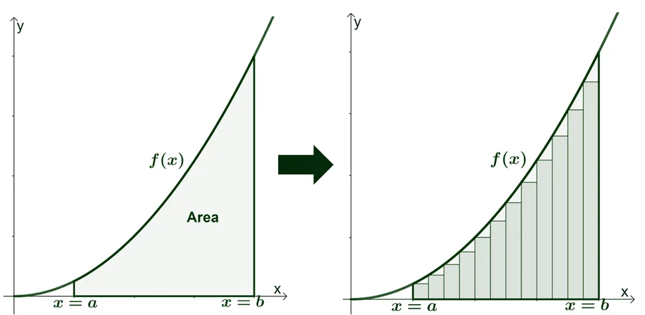
It works by dividing the interval into smaller subintervals, finding the area of rectangles over each subinterval, and adding them up.
The general form of a Riemann sum is:
\( \sum_{i=1}^{n} f(x_i^*) \cdot \Delta x \) where:
- \( f(x_i^*) \) is the function value at a chosen point in the subinterval (called a sample point)
- \( \Delta x \) is the width of each subinterval
- \( n \) is the number of subintervals
There are different types of Riemann sums depending on the sample point \( x_i^* \) used:
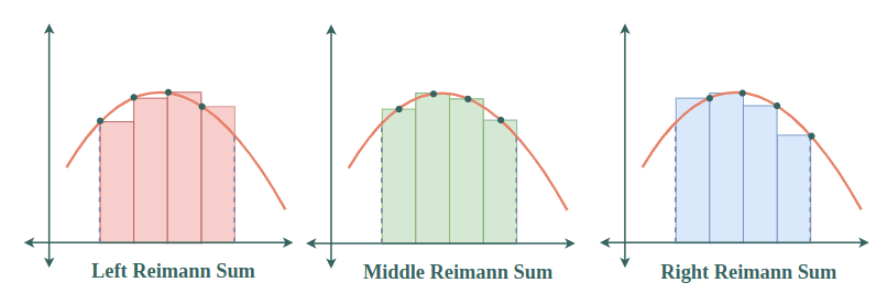
- Left Riemann Sum: uses the left endpoint of each subinterval
- Right Riemann Sum: uses the right endpoint of each subinterval
- Midpoint Riemann Sum: uses the midpoint of each subinterval
Summation Notation
Summation notation (also called sigma notation) is a concise way of writing long sums. It uses the Greek letter \( \Sigma \), which stands for “sum”.
A typical summation looks like this: \( \sum_{i=1}^{n} f(x_i) \)
This means:
“Add up the values of \( f(x_i) \) starting at \( i = 1 \) and ending at \( i = n \)”.
In Riemann sums, we often use summation notation to represent the total area: \( \sum_{i=1}^{n} f(x_i^*) \cdot \Delta x \) This tells us to multiply each function value by the width of the interval and sum over all subintervals.
Definite Integral Notation
The definite integral of a function \( f(x) \) from \( a \) to \( b \) is written using integral notation:
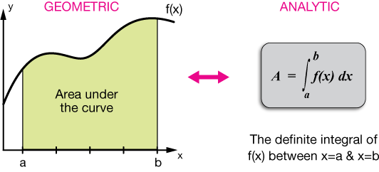
\( \displaystyle \int_a^b f(x) \, dx \)
Where:
- \( a \): Lower limit of integration
- \( b \): Upper limit of integration
- \( f(x) \): Function being integrated (rate of change)
- \( dx \): Indicates integration with respect to \( x \)
This notation represents the exact area under the curve \( f(x) \) from \( x = a \) to \( x = b \), and it is the limit of the Riemann sum as the number of rectangles \( n \to \infty \):
\( \displaystyle \int_a^b f(x)\,dx = \lim_{n \to \infty} \sum_{i=1}^n f(x_i^*) \cdot \Delta x \)
Example:
Estimate the area under the curve \( f(x) = x^2 + 1 \) from \( x = 0 \) to \( x = 4 \) using 4 rectangles and a Left Riemann Sum.
▶️Answer/Explanation
Divide the interval \([0,4]\) into 4 equal subintervals: width \( \Delta x = 1 \).
Left endpoints: \( x = 0, 1, 2, 3 \).
Evaluate:
\( f(0) = 1 \)
\( f(1) = 2 \)
\( f(2) = 5 \)
\( f(3) = 10 \)
Area ≈ \( \Delta x \cdot (f(0) + f(1) + f(2) + f(3)) = 1 \cdot (1 + 2 + 5 + 10) = 18 \).
Example:
Approximate the area under \( f(x) = \sin(x) \) on the interval \( [0, \pi] \) using 3 equal intervals and the midpoint rule.
▶️Answer/Explanation
Interval width: \( \Delta x = \dfrac{\pi}{3} \).
Midpoints: \( x = \dfrac{\pi}{6}, \dfrac{\pi}{2}, \dfrac{5\pi}{6} \).
Evaluate:
\( f\left(\dfrac{\pi}{6}\right) = \dfrac{1}{2} \)
\( f\left(\dfrac{\pi}{2}\right) = 1 \)
\( f\left(\dfrac{5\pi}{6}\right) = \dfrac{1}{2} \)
Area ≈ \( \Delta x \cdot \left( \dfrac{1}{2} + 1 + \dfrac{1}{2} \right) = \dfrac{\pi}{3} \cdot 2 = \dfrac{2\pi}{3} \approx 2.094 \)
Example:
Use summation notation to express the Right Riemann Sum approximation for \( f(x) = 3x + 2 \) over \( [1, 4] \) using 3 subintervals.
▶️Answer/Explanation
Subinterval width: \( \Delta x = 1 \).
Right endpoints: \( x_1 = 2, x_2 = 3, x_3 = 4 \).
Sum:
\( \sum_{i=1}^{3} f(x_i) \cdot \Delta x = (f(2) + f(3) + f(4)) \cdot 1 = (8 + 11 + 14) = 33 \).
So the Riemann sum is:
\( \sum_{i=1}^{3} f(x_i)\Delta x = 33 \).
Example:
Use 4 rectangles and a trapezoidal sum to approximate \( \displaystyle \int_{0}^{2} e^x dx \).
▶️Answer/Explanation
Subintervals: \( \Delta x = 0.5 \), at \( x = 0, 0.5, 1, 1.5, 2 \).
Evaluate function:
\( f(0) = 1 \),
\( f(0.5) \approx 1.649 \),
\( f(1) \approx 2.718 \),
\( f(1.5) \approx 4.481 \),
\( f(2) \approx 7.389 \).
Trapezoidal sum:
\( \dfrac{\Delta x}{2} \left[f(0) + 2f(0.5) + 2f(1) + 2f(1.5) + f(2)\right] \approx \dfrac{0.5}{2} (1 + 2(1.649) + 2(2.718) + 2(4.481) + 7.389) \)
$≈ 0.25 × (1 + 3.298 + 5.436 + 8.962 + 7.389) = 0.25 × 26.085 ≈ 6.521$
So, the approximate value of the integral is \( \boxed{6.521} \).