Modeling Situations with Differential Equations
Differential equations relate a function of an independent variable and the function’s derivatives. They are often used to model real-world situations where the rate of change of a quantity depends on the quantity itself or other variables.
A differential equation is an equation that involves an unknown function and its derivatives. For example,
\(\dfrac{dy}{dx} = ky\) is a first-order differential equation.
Types of Differential Equations:
| Type | Description |
| First-Order | Involves only the first derivative of the unknown function. |
| Second-Order | Involves the second derivative of the unknown function. |
| Linear | The dependent variable and its derivatives appear to the first power and are not multiplied together. |
| Nonlinear | The dependent variable or its derivatives appear to a power other than 1 or are multiplied together. |
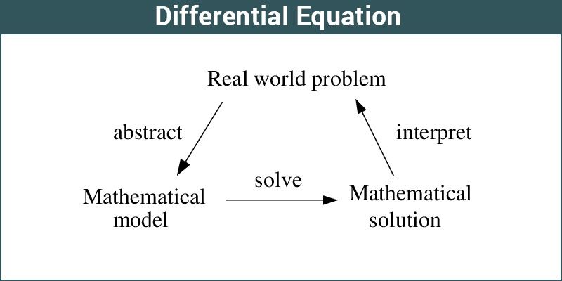
Steps for Modeling:
- Identify the variables and parameters in the problem.
- Establish a relationship between the rate of change and the variables involved.
- Write down the corresponding differential equation.
- Solve the equation (analytically or numerically) to find the function.
- Interpret the solution in the context of the problem.
Common Real-World Models:
- Exponential growth/decay: \(\dfrac{dy}{dt} = ky\)
- Newton’s Law of Cooling: \(\dfrac{dT}{dt} = -k(T – T_{\text{env}})\)
- Logistic growth: \(\dfrac{dy}{dt} = ky \left( 1 – \dfrac{y}{K} \right)\)
- Simple harmonic motion: \(\dfrac{d^2y}{dt^2} + \omega^2 y = 0\)
Example:
The rate of change of a population is proportional to its current size. The population doubles in 5 years. If the current population is 1,000, find the population after 8 years.
▶️Answer/Explanation
We model the situation as \(\dfrac{dP}{dt} = kP\).
Separating variables: \(\dfrac{dP}{P} = k\,dt\)
Integrating: \(\ln|P| = kt + C\) At \(t = 0, P = 1000\), so \(C = \ln 1000\).
The population doubles in 5 years: \(2000 = 1000 e^{5k} \Rightarrow e^{5k} = 2 \Rightarrow k = \dfrac{\ln 2}{5}\).
After 8 years: \(P(8) = 1000 e^{8 \cdot \frac{\ln 2}{5}} \approx 1000 \cdot 2^{8/5} \approx 3,031\).
Example:
A cup of coffee at 90°C is left in a room at 20°C. After 10 minutes, its temperature drops to 70°C. Find its temperature after 20 minutes.
▶️Answer/Explanation
Model: \(\dfrac{dT}{dt} = -k(T – 20)\)
Solution: \(T(t) = 20 + (T_0 – 20)e^{-kt}\)
Given \(T_0 = 90\) and \(T(10) = 70\): \(70 = 20 + 70e^{-10k} \Rightarrow e^{-10k} = \dfrac{50}{70} = \dfrac{5}{7}\)
So \(k = -\dfrac{1}{10} \ln \dfrac{5}{7}\)
After 20 minutes: \(T(20) = 20 + 70 e^{-20k} \approx 56.1^\circ\text{C}\)
Example:
A fish population in a lake follows the logistic equation \(\dfrac{dP}{dt} = 0.3P\left(1 – \dfrac{P}{500}\right)\), where \(t\) is in months. If \(P(0) = 50\), find \(P(5)\).
▶️Answer/Explanation
The logistic solution is \(P(t) = \dfrac{K}{1 + Ae^{-kt}}\), where \(K = 500, k = 0.3\).
From \(P(0) = 50\): \(50 = \dfrac{500}{1 + A} \Rightarrow A = 9\).
Thus \(P(t) = \dfrac{500}{1 + 9e^{-0.3t}}\).
At \(t = 5\): \(P(5) = \dfrac{500}{1 + 9e^{-1.5}} \approx 139.1\).