Sketching Slope Fields
A slope field (or direction field) is a graphical representation of the solutions to a first-order differential equation of the form:
\( \dfrac{dy}{dx} = f(x, y) \)
It consists of small line segments (or slopes) at various points \((x, y)\) in the plane, where the slope of each segment is given by \( f(x, y) \). These slope segments indicate the direction in which a solution curve would pass through that point.
Purpose of Slope Fields:
- To visualize the family of solution curves without solving the differential equation analytically.
- To understand the qualitative behavior of solutions over a region.
Steps to Sketch a Slope Field:
- Write the differential equation in the form \( \dfrac{dy}{dx} = f(x, y) \).
- Select a grid of points \((x, y)\) in the region of interest.
- At each point, calculate the slope \( m = f(x, y) \).
- Draw a short line segment through each point with slope \( m \).
- Optionally, sketch approximate solution curves by following the slope segments.
Special Cases:
- If \(m = 0\), draw a horizontal segment.
- If \(m > 0\), draw an upward-sloping segment.
- If \(m < 0\), draw a downward-sloping segment.
Key Idea: If \( \dfrac{dy}{dx} \) depends only on \( x \), the slopes are constant along vertical lines. If \( \dfrac{dy}{dx} \) depends only on \( y \), the slopes are constant along horizontal lines.
Mathematical Formulas:
- General form: \( \dfrac{dy}{dx} = f(x, y) \)
- For autonomous DEs: \( \dfrac{dy}{dx} = g(y) \) — slope depends only on \( y \)
- For separable DEs: \( \dfrac{dy}{dx} = g(y)h(x) \)
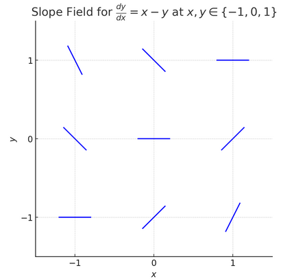
Example:
Sketch the slope field for \( \dfrac{dy}{dx} = x – y \) at the points \( x, y \in \{-1, 0, 1\} \).
▶️Answer/Explanation
Step 1: The slope formula is \( m = x – y \).
Step 2: Calculate slopes at each grid point:
| \( (x, y) \) | Slope \( m \) |
| \((-1, -1)\) | \( -1 – (-1) = 0 \) |
| \((-1, 0)\) | \( -1 – 0 = -1 \) |
| \((-1, 1)\) | \( -1 – 1 = -2 \) |
| \((0, -1)\) | \( 0 – (-1) = 1 \) |
| \((0, 0)\) | \( 0 – 0 = 0 \) |
| \((0, 1)\) | \( 0 – 1 = -1 \) |
| \((1, -1)\) | \( 1 – (-1) = 2 \) |
| \((1, 0)\) | \( 1 – 0 = 1 \) |
| \((1, 1)\) | \( 1 – 1 = 0 \) |
Step 3: At each grid point, draw a short segment with the corresponding slope.
The resulting slope field will guide us in sketching approximate solution curves.
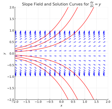
Example :
Describe the slope field for \( \dfrac{dy}{dx} = y \) and sketch several solution curves.
▶️Answer/Explanation
Here, \( m = y \) depends only on \( y \).
- For \( y = 0 \), slope \( m = 0 \) → horizontal segments.
- For \( y > 0 \), slope \( m > 0 \) → upward slant.
- For \( y < 0 \), slope \( m < 0 \) → downward slant.
Solution curves follow the exponential form \( y = Ce^x \) for various constants \( C \).
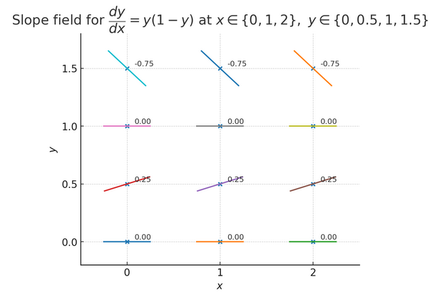
Example:
Sketch the slope field for:
\(\dfrac{dy}{dx} = y(1 – y)\)
Consider \(y \in \{0, 0.5, 1, 1.5\}\) and \(x \in \{0, 1, 2\}\).
▶️Answer/Explanation
The slope function is \(m = y(1 – y)\).
Key features:
- When \(y = 0\) or \(y = 1\), slope is 0 → horizontal segments.
- If \(0 < y < 1\), slope is positive → upward segments.
- If \(y > 1\), slope is negative → downward segments.
This indicates two equilibrium solutions: \(y = 0\) and \(y = 1\).