Reasoning Using Slope Fields
A slope field (or direction field) is a graphical representation of the slopes of the tangent lines to the solution curves of a first-order differential equation without explicitly solving it.
Given a differential equation of the form:
\( \dfrac{dy}{dx} = f(x, y) \)
At each point \((x, y)\) in the plane, a small line segment is drawn with slope \( f(x, y) \). These segments help visualize how the solutions behave.

Reasoning with slope fields involves using these visual cues to:
- Predict the shape of solution curves without solving the equation analytically.
- Identify equilibrium solutions (where \( \dfrac{dy}{dx} = 0 \)).
- Determine the qualitative behavior of solutions (e.g., growth, decay, oscillations).
Key Points:
- Horizontal segments indicate zero slope (\( \dfrac{dy}{dx} = 0 \)), often corresponding to constant solutions.
- Positive slopes indicate an increasing solution curve.
- Negative slopes indicate a decreasing solution curve.
- Different initial conditions can lead to different solution curves in the same slope field.
Example:
Consider the differential equation:
\( \dfrac{dy}{dx} = x – y \)
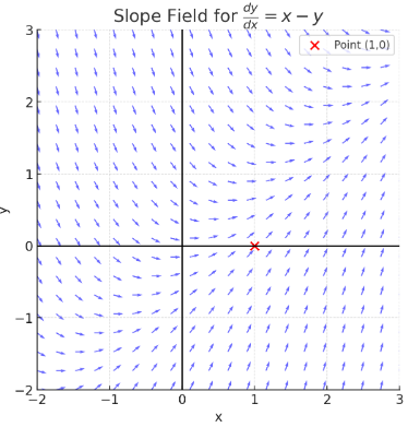
Using the slope field, determine whether the solution curves are increasing or decreasing near the point \( (1, 0) \).
▶️Answer/Explanation
At \( (1, 0) \), we have: \( \dfrac{dy}{dx} = 1 – 0 = 1 \) This slope is positive, so the solution curve is increasing near \( (1, 0) \).
Example:
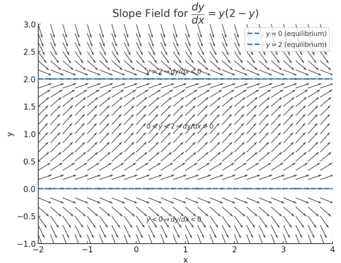
The slope field for the equation \( \dfrac{dy}{dx} = y(2 – y) \) shows horizontal segments along \( y = 0 \) and \( y = 2 \).
What can you conclude?
▶️Answer/Explanation
When \( y = 0 \) or \( y = 2 \), we have: \( \dfrac{dy}{dx} = 0 \) Thus, these are equilibrium solutions. The slope field shows that:
- For \( 0 < y < 2 \), slopes are positive, so solutions increase toward \( y = 2 \).
- For \( y > 2 \) or \( y < 0 \), slopes are negative, so solutions move toward these equilibria from above or below.
Example :
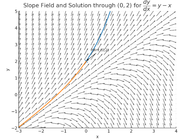
Without solving, use the slope field for \( \dfrac{dy}{dx} = y – x \) to describe the behavior of the solution passing through \( (0, 2) \).
▶️Answer/Explanation
At \( (0, 2) \), slope is: \( \dfrac{dy}{dx} = 2 – 0 = 2 \) The slope is positive, so the solution curve rises steeply. As \( x \) increases, the slope decreases when \( y \) approaches \( x \), eventually becoming zero when \( y = x \). Past that, the slope turns negative.