Exponential Models with Differential Equations
Exponential models describe situations where the rate of change of a quantity is proportional to the quantity itself. These are common in contexts such as population growth, radioactive decay, cooling, and finance. Such models can be expressed as first-order differential equations.
The general form is:
\(\dfrac{dy}{dt} = ky\)
where:
- \(y\) is the quantity at time \(t\)
- \(k\) is the constant of proportionality
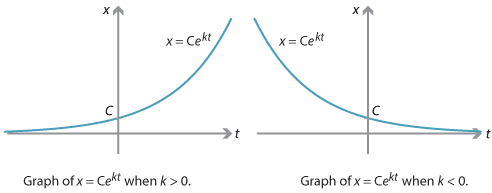
- \(k > 0\) models exponential growth
- \(k < 0\) models exponential decay
Solution to the General Exponential Model:
Solving \(\dfrac{dy}{dt} = ky\) by separation of variables:
\( \frac{1}{y} \, dy = k \, dt \) Integrating: \( \ln|y| = kt + C \)
Exponentiating: \( y = Ae^{kt} \) where \(A\) is a constant determined by initial conditions.
Key Notes:
- If \(y(0) = y_0\), then \(A = y_0\) and the solution is: \( y = y_0 e^{kt} \)
- The sign of \(k\) determines growth (\(k > 0\)) or decay (\(k < 0\)).
- Half-life, doubling time, and other time constants can be found using logarithmic properties.
Procedure for Solving Exponential Models:
- Write the problem as a differential equation of the form \(\dfrac{dy}{dt} = ky\).
- Separate variables and integrate to find the general solution \(y = Ae^{kt}\).
- Apply the given initial condition to find \(A\).
- If a second data point is given, use it to determine \(k\).
Example:
A population of bacteria grows at a rate proportional to its size. Initially, there are 500 bacteria, and after 3 hours the population reaches 2000. Find the population at any time \(t\).
▶️Answer/Explanation
Let \(y\) be the population at time \(t\) hours.
We have:
\( \frac{dy}{dt} = ky \)
General solution:
\( y = Ae^{kt} \)
From
\(y(0) = 500\): \( 500 = Ae^{0} \quad \Rightarrow \quad A = 500 \)
So:
\( y = 500 e^{kt} \)
From \(y(3) = 2000\):
\( 2000 = 500 e^{3k} \quad \Rightarrow \quad 4 = e^{3k} \quad \Rightarrow \quad 3k = \ln 4 \quad \Rightarrow \quad k = \frac{\ln 4}{3} \)
Thus:
\( y = 500 e^{\left(\frac{\ln 4}{3}\right) t} \)
Example:
A radioactive substance decays at a rate proportional to its mass. Initially, there are 100 g, and after 10 hours, 25 g remain. Find the formula for the mass \(m(t)\) at time \(t\).
▶️Answer/Explanation
We have:
\( \frac{dm}{dt} = km \)
General solution:
\( m = Ae^{kt} \)
From \(m(0) = 100\):
\( 100 = A \quad \Rightarrow \quad m = 100 e^{kt} \)
From \(m(10) = 25\):
\( 25 = 100 e^{10k} \quad \Rightarrow \quad 0.25 = e^{10k} \quad \Rightarrow \quad 10k = \ln(0.25) \quad \Rightarrow \quad k = \frac{\ln(0.25)}{10} \)
Thus:
\( m(t) = 100 e^{\left(\frac{\ln(0.25)}{10}\right) t} \)
Example:
The mass of a certain radioactive isotope decreases at a rate proportional to its mass. Initially, the mass is 120 g. After 5 years, the mass is 90 g. Which of the following represents the mass \(m(t)\) at time \(t\) years?
- \(m(t) = 120 e^{\frac{\ln(3/4)}{5}t}\)
- \(m(t) = 120 e^{\frac{\ln(4/3)}{5}t}\)
- \(m(t) = 120 e^{\frac{\ln(2/3)}{5}t}\)
- \(m(t) = 120 e^{\frac{\ln(3/2)}{5}t}\)
▶️Answer/Explanation
We start with: \( \frac{dm}{dt} = km \)
General solution: \( m(t) = Ae^{kt} \)
From \(m(0) = 120\), \(A = 120\): \( m(t) = 120 e^{kt} \)
From \(m(5) = 90\): \( 90 = 120 e^{5k} \quad \Rightarrow \quad \frac{3}{4} = e^{5k} \quad \Rightarrow \quad 5k = \ln\left(\frac{3}{4}\right) \)
\( k = \frac{\ln(3/4)}{5} \)
So: \( m(t) = 120 e^{\left(\frac{\ln(3/4)}{5}\right)t} \)
Correct answer: A.