AP Calculus BC 7.9 Logistic Models with Differential Equations Study Notes - New Syllabus

Logistic Models with Differential Equations

The logistic growth model describes situations where a population or quantity grows rapidly at first but slows as it approaches a maximum sustainable value, known as the carrying capacity. This type of growth occurs in many real-world situations, such as population growth in limited environments, spread of diseases, or chemical reactions with limited resources.

General Logistic Differential Equation:

The model can be expressed as:

\(\dfrac{dy}{dt} = k \, y \, (a – y)\)

Here:

• \(y\) = the quantity or population size at time \(t\)
• \(a\) = carrying capacity (maximum possible value of \(y\))
• \(k > 0\) = proportionality constant
• \(\dfrac{dy}{dt}\) = rate of change of \(y\) with respect to time

Meaning of the Model:

The equation states that:

• The rate of change is proportional to \(y\) (the current size) — larger populations tend to grow faster initially.
• The rate of change is also proportional to \((a – y)\), which is the difference between the carrying capacity and the current size — growth slows as \(y\) gets closer to \(a\).
• When \(y = 0\) or \(y = a\), the rate of change is zero, meaning no growth.

Solution to the Logistic Differential Equation:

Using separation of variables and integration, the general solution is:

\(y(t) = \dfrac{a}{1 + Ce^{-akt}}\)

where \(C\) is determined by initial conditions.

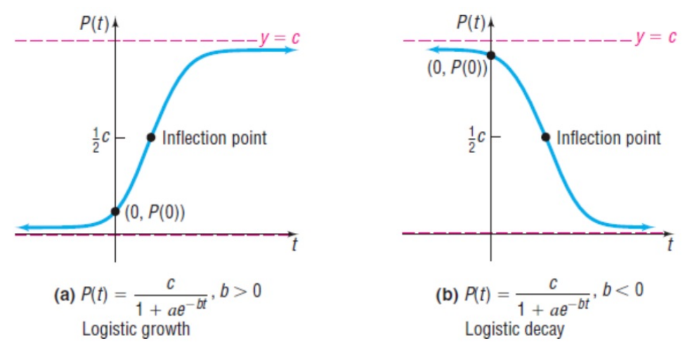
Features of Logistic Growth:

• Initial rapid growth: When \(y\) is small compared to \(a\), growth is approximately exponential.
• Slowing growth: As \(y\) approaches \(a\), growth rate decreases.
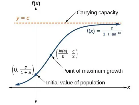
• Point of fastest growth: Occurs when \(y = \dfrac{a}{2}\).
• Equilibrium values: \(y = 0\) and \(y = a\) are stable states.

More AP Calculus Concepts:

The logistic differential equation and initial conditions can be interpreted without solving the equation.

• • By analyzing the equation \(\dfrac{dy}{dt} = k y (a – y)\), one can determine whether the quantity is increasing or decreasing at any given \(y\).
  • If \(0 < y < a\), the rate is positive (growth). If \(y > a\), the rate is negative (decay).
  • Initial conditions tell us the starting position on the logistic curve and how the quantity will evolve over time.

 The limiting value (carrying capacity) can be found without solving.

• • From the equation, when \(t \to \infty\), \(y \to a\).
  • This limit is independent of initial conditions (as long as \(y > 0\) and less than \(a\)).

The point of fastest change occurs when \(y = \dfrac{a}{2}\).

• • The derivative \(\dfrac{dy}{dt} = k y (a – y)\) is a quadratic in \(y\), with maximum at \(y = \dfrac{a}{2}\).
  • At this point, growth rate is maximized and equals \(\dfrac{ka^2}{4}\).