AP Physics 1- 2.2 Forces and Free-Body Diagrams - Exam Style questions - FRQs- New Syllabus

(a)(i)
The acceleration is approximately \( \boxed{0} \), or extremely small.

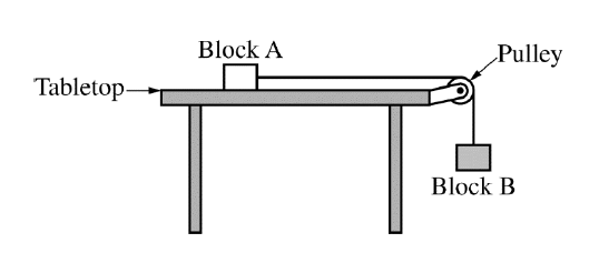
If block \( A \) is much more massive than block \( B \), then block \( A \) has a very large inertia and is hard to accelerate. The hanging block is too light to produce much motion, so the whole system accelerates only a tiny amount.

In words: the heavy block on the table is so difficult to speed up that the system barely moves.

(a)(ii)
The acceleration is approximately \( \boxed{g} \) \( \big(\text{or about } 9.8\ \mathrm{m/s^2}\big) \).

If block \( A \) is much less massive than block \( B \), then block \( A \) offers very little resistance to the motion. The hanging block behaves almost like a freely falling mass, so the acceleration approaches \( g \).

It is not exactly equal to \( g \) unless the other mass becomes negligible, but it gets very close.

(b)
The correct free-body diagrams are:

For block \( A \):
\( \bullet \) Normal force \( F_N \) upward
\( \bullet \) Gravitational force \( F_g \) downward
\( \bullet \) Tension force \( F_T \) horizontally to the right

For block \( B \):
\( \bullet \) Tension force \( F_T \) upward
\( \bullet \) Gravitational force \( F_g \) downward

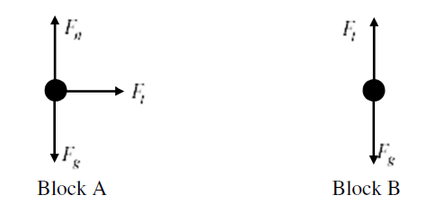
There is no friction force on block \( A \), because the tabletop is stated to have negligible friction.

(c)
Apply Newton’s second law separately to each block.

For block \( A \) \( (\text{horizontal direction}) \):

\( F_T = m_A a \)

For block \( B \) \( (\text{taking downward as positive}) \):

\( m_B g – F_T = m_B a \)

Substitute \( F_T = m_A a \) into the equation for block \( B \):

\( m_B g – m_A a = m_B a \)

\( m_B g = m_A a + m_B a \)

\( m_B g = (m_A + m_B)a \)

Solve for \( a \):

\( \boxed{a = \dfrac{m_B}{m_A + m_B}\,g} \)

This expression makes good physical sense: increasing \( m_B \) makes the pull stronger, while increasing either mass increases the inertia of the moving system.

(d)
\( \boxed{\text{Yes}} \)

The equation from part \( \mathrm{(c)} \) is \( a = \dfrac{m_B}{m_A + m_B}g \). When \( m_A \ll m_B \), the term \( m_A \) is negligible compared with \( m_B \), so

\( a \approx \dfrac{m_B}{m_B}g = g \)

Therefore the equation predicts that the acceleration approaches \( g \), which matches the reasoning in part \( \mathrm{(a)(ii)} \).

(e)
\( \boxed{T_2 > T_1} \)

When the pulley has nonnegligible mass, some of the net force effect goes into rotating the pulley as well as accelerating the blocks. That makes the acceleration of the blocks smaller than before.

For block \( B \), the forces are weight downward and tension upward. If the downward acceleration becomes smaller while \( m_B g \) stays the same, then the upward tension must be larger. So the tension in the vertical part of the string is greater with the massive pulley.

In other words, a rotationally inert pulley reduces the system’s acceleration, which means the hanging block’s net downward force is smaller, so the tension has to be closer to the block’s weight.