AP Physics 1- 1.3 Representing Motion - Exam Style questions - FRQs- New Syllabus
Representing Motion AP Physics 1 FRQ
Unit: 1. Kinematics
Weightage : 10-15%
Question

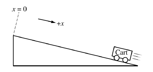
Students conduct an experiment to determine the acceleration \( a \) of a cart. The cart is released from rest at the top of a ramp at time \( t=0 \) and moves down the ramp. The \( x \)-axis is defined to be parallel to the ramp with its origin at the top, as shown in the figure. The students collect the data shown in the following table.
| Position \( x \) \( (\mathrm{m}) \) | Time \( t \) \( (\mathrm{s}) \) | ||
|---|---|---|---|
| \( 0.06 \) | \( 0.39 \) | ||
| \( 0.14 \) | \( 0.59 \) | ||
| \( 0.24 \) | \( 0.77 \) | ||
| \( 0.37 \) | \( 0.96 \) | ||
| \( 0.55 \) | \( 1.20 \) |


Most-appropriate topic codes (AP Physics 1):
• Topic \( 2.5 \) — Newton’s Second Law (Part \( \mathrm{(b)} \), Part \( \mathrm{(c)} \))
• Topic \( 2.6 \) — Gravitational Force (Part \( \mathrm{(b)} \), Part \( \mathrm{(c)} \))
• Topic \( 3.A \) / Experimental Design (Part \( \mathrm{(a)} \), Part \( \mathrm{(b)} \), Part \( \mathrm{(c)} \))
▶️ Answer/Explanation
(a)(i)
Since the cart is released from rest and has constant acceleration down the ramp,
\( x = \dfrac{1}{2}at^2 \)
Therefore, a graph of position versus time squared is linear.
Vertical axis: \( x\ (\mathrm{m}) \)
Horizontal axis: \( t^2\ (\mathrm{s^2}) \)
| Position \( x \) \( (\mathrm{m}) \) | Time \( t \) \( (\mathrm{s}) \) | Time squared \( t^2 \) \( (\mathrm{s^2}) \) |
|---|---|---|
| \( 0.06 \) | \( 0.39 \) | \( 0.15 \) |
| \( 0.14 \) | \( 0.59 \) | \( 0.35 \) |
| \( 0.24 \) | \( 0.77 \) | \( 0.59 \) |
| \( 0.37 \) | \( 0.96 \) | \( 0.92 \) |
| \( 0.55 \) | \( 1.20 \) | \( 1.44 \) |
(a)(ii)
Plot the points \( (0.15,0.06) \), \( (0.35,0.14) \), \( (0.59,0.24) \), \( (0.92,0.37) \), and \( (1.44,0.55) \) on a graph of \( x \) versus \( t^2 \), and draw a straight best-fit line.
A correct graph should look approximately like this:

(a)(iii)
The slope of the best-fit line is approximately
\( \text{slope} = \dfrac{\Delta x}{\Delta t^2} \approx 0.375\ \mathrm{\dfrac{m}{s^2}} \)
Using \( x = \dfrac{1}{2}at^2 \), the slope of the graph is \( \dfrac{1}{2}a \).
Therefore,
\( a = 2(\text{slope}) = 2(0.375) \)
\( \boxed{a \approx 0.75\ \mathrm{m/s^2}} \)
Any nearby value from a reasonable best-fit line earns credit.
(b)(i)
The students must measure either:
\( \bullet \) the angle \( \theta \) that the ramp makes with the horizontal, or
\( \bullet \) the height \( h \) and length \( L \) of the ramp
so that they can relate the component of gravity along the ramp to the measured acceleration.
(b)(ii)
Along the ramp,
\( mg_{\mathrm{exp}}\sin\theta = ma \)
so
\( \boxed{g_{\mathrm{exp}} = \dfrac{a}{\sin\theta}} \)
Equivalently, if \( \sin\theta = \dfrac{h}{L} \), then
\( \boxed{g_{\mathrm{exp}} = \dfrac{L}{h}a} \)
(c)(i)
One valid physical reason is that the wheels of the cart may have nonnegligible rotational inertia.
Other acceptable ideas include a bad angle measurement, a bumpy ramp, a nonlevel setup, or another physical measurement issue.
(c)(ii)
If the wheels have rotational inertia, some of the gravitational effect goes into making the wheels rotate instead of producing translational acceleration of the cart’s center of mass.
That means the measured acceleration \( a \) would be smaller than the ideal value \( g\sin\theta \). Since \( g_{\mathrm{exp}} \) is calculated from \( a \), the smaller measured acceleration leads to a smaller calculated value of \( g_{\mathrm{exp}} \), making it lower than \( 9.8\ \mathrm{m/s^2} \).
(d)
While the cart moves up the ramp, the acceleration is still constant and directed down the ramp \( (+x) \).
Therefore:
\( \bullet \) The graph of \( x \) versus \( t \) is a concave-up curve with an initially negative slope. The cart begins at a positive position near the bottom, moves upward toward the origin at the top, and momentarily comes to rest, so the slope increases from negative toward zero.
\( \bullet \) The graph of \( v \) versus \( t \) is a straight line with positive slope and a negative vertical intercept. The cart starts with negative velocity \( (\text{moving up the ramp, opposite } +x) \) and then the velocity increases linearly to \( 0 \).
A correct sketch is like this:
