Home / AP® Exam / AP® Physics C: Electricity and Magnetism / AP Physics C E&M – 12.4 Ampère’s Law- Study Notes

AP Physics C E&M- 12.4 Ampère’s Law- Study Notes- New Syllabus

AP Physics C E&M- 12.4 Ampère’s Law – Study Notes

AP Physics C E&M- 12.4 Ampère’s Law – Study Notes – per latest Syllabus.

Key Concepts:

  • Ampère’s Law and Magnetic Fields from Moving Charges
  • Maxwell’s Fourth Equation: Ampère’s Law with Maxwell’s Addition

AP Physics C E&M-Concise Summary Notes- All Topics

Ampère’s Law and Magnetic Fields from Moving Charges

Ampère’s law relates the integrated magnetic field around a closed loop to the total current passing through the surface enclosed by that loop. It is one of Maxwell’s equations.

Ampère’s Law (Integral Form):  

\( \mathrm{\oint \vec{B} \cdot d\vec{\ell} = \mu_0 I_{enc}} \)

  • \(\mathrm{\vec{B}}\) = magnetic field
  • \(\mathrm{d\vec{\ell}}\) = infinitesimal length element of the loop
  • \(\mathrm{I_{enc}}\) = net current enclosed by the loop
  • \(\mathrm{\mu_0 = 4\pi \times 10^{-7} \, T \cdot m/A}\)

Magnetic Field from a Long Straight Wire:

For a wire carrying current \(I\), consider a circular Ampèrian loop of radius \(r\):

\( \mathrm{B (2 \pi r) = \mu_0 I} \quad \Rightarrow \quad B = \dfrac{\mu_0 I}{2 \pi r}} \)

  • The field decreases as \(1/r\).
  • Direction given by the right-hand rule (thumb = current, curled fingers = \(\vec{B}\)).

Magnetic Field Inside a Current-Carrying Cylinder:

Uniform current distribution, radius \(R\), total current \(I\).
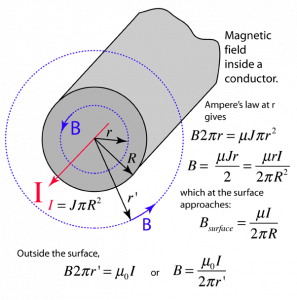
  • For \(r < R\):

    \( \mathrm{B (2 \pi r) = \mu_0 I_{enc}} \), where \(\mathrm{I_{enc} = I \dfrac{r^2}{R^2}} \).

    \( \mathrm{B = \dfrac{\mu_0 I r}{2 \pi R^2}} \)

  • For \(r \geq R\):

    \( \mathrm{B = \dfrac{\mu_0 I}{2 \pi r}} \)

Magnetic Field in a Solenoid (Application of Ampère’s Law):

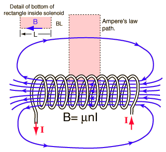
Inside a solenoid with \(n\) turns per unit length carrying current \(I\):

\( \mathrm{B = \mu_0 n I} \)

  • The field inside is uniform and parallel to the solenoid’s axis.
  • Outside, the field is nearly zero (for an ideal solenoid).

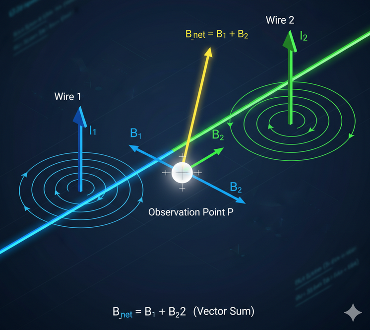
Principle of Superposition:

Magnetic fields are vectors; the net field at any point is the vector sum of fields from all sources.

  • This allows calculation of fields from:
    • Multiple current-carrying wires.
    • Circular loops or coils.
    • Segments of wires or cylindrical conductors.

Key Idea: Ampère’s law is a powerful tool to calculate magnetic fields in symmetric situations, while superposition is used when multiple sources contribute to the total field.

Example :

Use Ampère’s law to find the magnetic field at a point \(4.0 \, cm\) away from a long wire carrying a current of \(10 \, A\).

▶️ Answer/Explanation

Step 1: Ampère’s law: \( \mathrm{B (2 \pi r) = \mu_0 I} \).

Step 2: Solve for \(B\): \( \mathrm{B = \dfrac{\mu_0 I}{2 \pi r}} \).

Step 3: Substitute values: \( \mathrm{B = \dfrac{(4\pi \times 10^{-7})(10)}{2 \pi (0.04)}} \).

Step 4: \( \mathrm{B = 5.0 \times 10^{-5} \, T} \).

Final Answer: The magnetic field is \( \mathrm{5.0 \times 10^{-5} \, T} \), directed circularly around the wire.

Example:

Two parallel wires, each carrying current \(I = 5.0 \, A\), are separated by \(0.10 \, m\). Find the net magnetic field at a point midway between them if currents are in opposite directions.

▶️ Answer/Explanation

Step 1: Field due to one wire at midpoint: \( \mathrm{B = \dfrac{\mu_0 I}{2 \pi r}} \), with \( r = 0.05 \, m \).

Step 2: \( \mathrm{B = \dfrac{(4\pi \times 10^{-7})(5.0)}{2 \pi (0.05)}} = 2.0 \times 10^{-5} \, T \).

Step 3: Because currents are opposite, their fields at the midpoint add.

Step 4: Net field = \( 2 (2.0 \times 10^{-5}) = 4.0 \times 10^{-5} \, T \).

Final Answer: The net magnetic field at the midpoint is \( \mathrm{4.0 \times 10^{-5} \, T} \).

Maxwell’s Fourth Equation: Ampère’s Law with Maxwell’s Addition

 Maxwell’s equations form the foundation of electromagnetism. The fourth equation is the Ampère–Maxwell law, which extends Ampère’s law by including the effect of a changing electric field.

Integral Form:

\( \mathrm{\oint \vec{B} \cdot d\vec{\ell} = \mu_0 I_{enc} + \mu_0 \varepsilon_0 \dfrac{d\Phi_E}{dt}} \)

  • \(\mathrm{\vec{B}}\) = magnetic field
  • \(\mathrm{d\vec{\ell}}\) = infinitesimal element along the closed loop
  • \(\mathrm{I_{enc}}\) = conduction current enclosed by the loop
  • \(\mathrm{\varepsilon_0}\) = permittivity of free space
  • \(\mathrm{\dfrac{d\Phi_E}{dt}}\) = rate of change of electric flux through the surface

Differential Form:

\( \mathrm{\nabla \times \vec{B} = \mu_0 \vec{J} + \mu_0 \varepsilon_0 \dfrac{\partial \vec{E}}{\partial t}} \)

  • \(\mathrm{\vec{J}}\) = current density
  • The second term is the displacement current density: \( \mathrm{J_D = \varepsilon_0 \dfrac{\partial \vec{E}}{\partial t}} \)

Physical Meaning:

  • Ampère’s contribution: A steady electric current (\(I\)) produces a magnetic field.
  • Maxwell’s addition: A time-varying electric field (\(\dfrac{\partial \vec{E}}{\partial t}\)) also produces a magnetic field, even in regions without conduction current.
  • This resolves inconsistencies in Ampère’s law, especially in cases like charging capacitors.

Example: Charging Capacitor

  • Between the plates of a charging capacitor, no conduction current flows.
  • But the changing electric field between the plates (\(\dfrac{d\Phi_E}{dt}\)) produces a displacement current.
  • This ensures continuity of magnetic fields around the capacitor, consistent with Maxwell’s law.

Key Idea: Magnetic fields can be generated by both conduction currents and changing electric fields. This concept is essential to the existence of electromagnetic waves.

Example :

A parallel-plate capacitor has plate area \(0.01 \, m^2\) and plate separation \(1.0 \times 10^{-3} \, m\). The capacitor is being charged so that the electric field between the plates increases at a rate of \(2.0 \times 10^{12} \, V/m \cdot s\). Find the displacement current between the plates.

▶️ Answer/Explanation

Step 1: Displacement current: \( \mathrm{I_D = \varepsilon_0 \dfrac{d\Phi_E}{dt}} \).

Step 2: Electric flux: \( \mathrm{\Phi_E = E \cdot A} \).

Step 3: Rate of change: \( \mathrm{\dfrac{d\Phi_E}{dt} = A \dfrac{dE}{dt}} = (0.01)(2.0 \times 10^{12}) = 2.0 \times 10^{10} \, V \cdot m \).

Step 4: Substitute: \( \mathrm{I_D = (8.85 \times 10^{-12})(2.0 \times 10^{10})} \).

Step 5: \( \mathrm{I_D = 0.177 \, A} \).

Final Answer: The displacement current is \( \mathrm{0.18 \, A} \).

Scroll to Top