Electric Potential Due to a Configuration of Charged Objects
The electric potential at a point in space is the electric potential energy per unit charge that a positive test charge would have at that point. It is a scalar quantity, unlike the electric field, which is a vector.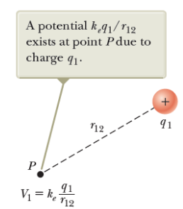
Electric Potential Due to a Point Charge:
\( \mathrm{V = \dfrac{1}{4 \pi \varepsilon_0} \dfrac{q}{r}} \)
- \(\mathrm{V}\) = electric potential (volts, \( \mathrm{J/C} \))
- \(\mathrm{q}\) = source charge
- \(\mathrm{r}\) = distance from the charge
Superposition Principle:
For a configuration of multiple point charges, the total potential at a point is the sum of potentials from each charge:
\( \mathrm{V_{total} = \sum_i V_i = \dfrac{1}{4 \pi \varepsilon_0} \sum_i \dfrac{q_i}{r_i}} \)
- Unlike electric field vectors, potentials add algebraically (scalar superposition).
Continuous Charge Distributions: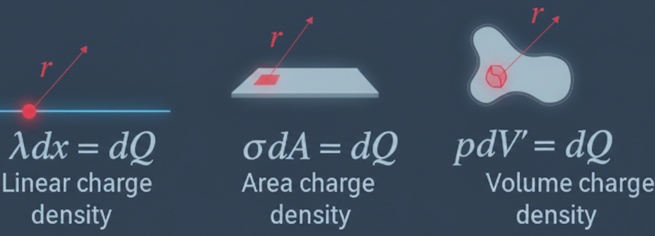
If charges are distributed continuously, the potential is obtained using integration:
\( \mathrm{V = \dfrac{1}{4 \pi \varepsilon_0} \displaystyle \int \dfrac{dq}{r}} \)
- For line charge: \( dq = \lambda \, dl \)
- For surface charge: \( dq = \sigma \, dA \)
- For volume charge: \( dq = \rho \, dV \)
Electric Potential Difference: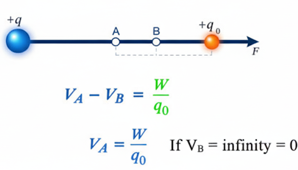
The potential difference between two points A and B is the change in potential energy per unit charge when moving a test charge:
\( \mathrm{\Delta V = V_B – V_A = \dfrac{U_B – U_A}{q_{test}} = -\displaystyle \int_A^B \vec{E} \cdot d\vec{l}} \)
- A positive \(\Delta V\) means the test charge has gained potential energy.
- A negative \(\Delta V\) means the test charge has lost potential energy (field does positive work).
Other Sources of Potential Difference:
- Electric potential differences can also arise from chemical processes that separate positive and negative charges, such as in a battery.
- This creates an electric field that drives current in circuits.
Example:
Find the electric potential at a point \(0.3 \, m\) from a charge \(+2.0 \, \mu C\) and \(0.4 \, m\) from a charge \(-1.0 \, \mu C\).
▶️ Answer/Explanation
Step 1: Potential due to first charge: \( \mathrm{V_1 = \dfrac{1}{4 \pi \varepsilon_0} \dfrac{q_1}{r_1}} \) \( \mathrm{V_1 = (9 \times 10^9) \dfrac{2.0 \times 10^{-6}}{0.3}} \approx 6.0 \times 10^4 \, V} \)
Step 2: Potential due to second charge: \( \mathrm{V_2 = (9 \times 10^9) \dfrac{-1.0 \times 10^{-6}}{0.4}} \approx -2.25 \times 10^4 \, V} \)
Step 3: Total potential: \( \mathrm{V_{total} = V_1 + V_2 = 6.0 \times 10^4 – 2.25 \times 10^4 = 3.75 \times 10^4 \, V} \)
Final Answer: \( \mathrm{V = 3.75 \times 10^4 \, V} \).
Example:
A charge \(Q = +5.0 \, \mu C\) creates an electric potential. What is the potential difference between points at distances \(0.5 \, m\) and \(1.0 \, m\) from the charge?
▶️ Answer/Explanation
Step 1: Potential at \(r_1 = 0.5 \, m\): \( \mathrm{V_1 = \dfrac{1}{4 \pi \varepsilon_0} \dfrac{Q}{r_1}} \) \( \mathrm{V_1 = (9 \times 10^9) \dfrac{5.0 \times 10^{-6}}{0.5} = 9.0 \times 10^4 \, V} \)
Step 2: Potential at \(r_2 = 1.0 \, m\): \( \mathrm{V_2 = (9 \times 10^9) \dfrac{5.0 \times 10^{-6}}{1.0} = 4.5 \times 10^4 \, V} \)
Step 3: Potential difference: \( \mathrm{\Delta V = V_2 – V_1 = 4.5 \times 10^4 – 9.0 \times 10^4 = -4.5 \times 10^4 \, V} \)
Final Answer: \( \mathrm{\Delta V = -4.5 \times 10^4 \, V} \), meaning a positive test charge loses potential energy moving outward.
Example :
A uniformly charged ring has total charge \( \mathrm{Q = 5.0 \times 10^{-6} \, C} \) and radius \( \mathrm{R = 0.10 \, m} \). Find the electric potential at a point on the axis a distance \( \mathrm{x = 0.20 \, m} \) from the center of the ring.
▶️ Answer/Explanation
Step 1: For a uniformly charged ring, every charge element is the same distance \( \mathrm{r = \sqrt{R^2 + x^2}} \) from the point on the axis. By superposition (and symmetry) the potential is
\( \mathrm{V = \dfrac{1}{4\pi\varepsilon_0}\dfrac{Q}{\sqrt{R^2 + x^2}}} \)
Step 2: Substitute values (\( \mathrm{\dfrac{1}{4\pi\varepsilon_0} \approx 9.0 \times 10^9 \, N\,m^2/C^2} \)):
\( \mathrm{V = (9.0 \times 10^9)\dfrac{5.0 \times 10^{-6}}{\sqrt{(0.10)^2 + (0.20)^2}}} \)
Step 3: Calculate the denominator: \( \mathrm{R^2 + x^2 = 0.01 + 0.04 = 0.05 \, m^2} \), so \( \mathrm{\sqrt{R^2+x^2} = 0.2236 \, m} \).
Step 4: Compute the potential:
\( \mathrm{V \approx \dfrac{(9.0 \times 10^9)(5.0 \times 10^{-6})}{0.2236} \approx \dfrac{4.50 \times 10^4}{0.2236} \approx 2.01 \times 10^5 \, V} \)
Final Answer: The electric potential at the point on the axis is approximately \( \mathrm{2.01 \times 10^5 \, V} \).
Relationship Between Electric Potential and Electric Field
The electric field is related to the rate of change of electric potential with position. The field points in the direction of greatest decrease of potential.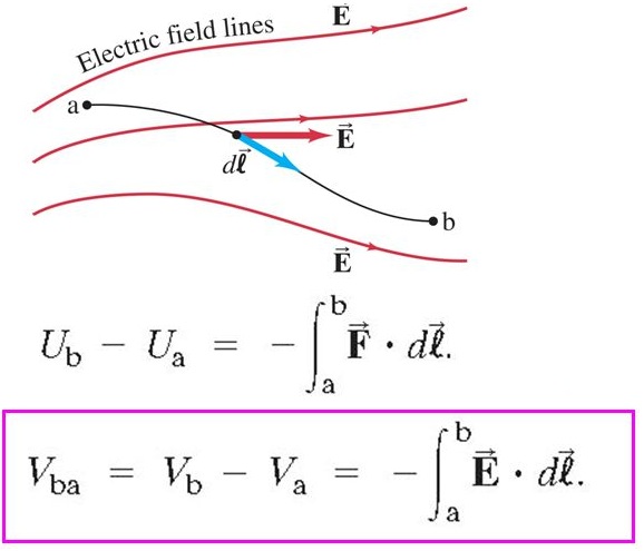
Mathematical Relation:
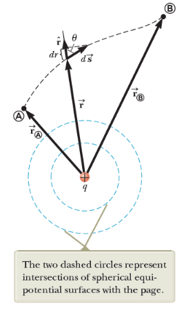
The change in potential between two points A and B is the negative line integral of the electric field along the path:
\( \mathrm{\Delta V = V_B – V_A = -\displaystyle \int_A^B \vec{E} \cdot d\vec{l}} \)
In one dimension (uniform field along x):
\( \mathrm{E_x = – \dfrac{dV}{dx}} \)
Interpretation:
- A strong electric field corresponds to a rapid change in potential.
- The field points from higher potential to lower potential.
Equipotential Lines and Surfaces:
Equipotential lines (2D) or equipotential surfaces (3D) are sets of points with the same electric potential (also called isolines).
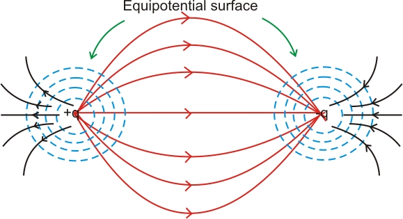
Properties:
- Always perpendicular to electric field lines.
- No work is required to move a charge along an equipotential line (since \(\mathrm{\Delta V = 0}\)).
- Closer spacing of equipotential lines indicates stronger electric fields.
- Equipotentials around:
- Point charges → concentric spheres (3D).
- Parallel plate capacitor → parallel planes.
Applications:
- Visualizing the relationship between electric potential and electric field.
- Predicting motion of charges (positive charges move toward lower potential, negative charges toward higher potential).
Example :
A uniform electric field of \( \mathrm{E = 200 \, N/C} \) points along the +x axis. Find the potential difference between two points separated by \( \mathrm{0.5 \, m} \) along the x-axis.
▶️ Answer/Explanation
Step 1: Relation between potential difference and field: \( \mathrm{\Delta V = – E \Delta x} \)
Step 2: Substitute values: \( \mathrm{\Delta V = – (200)(0.5)} \)
Step 3: \( \mathrm{\Delta V = -100 \, V} \)
Final Answer: The potential decreases by \( \mathrm{100 \, V} \) in the direction of the electric field.