AP Physics C- E&M- 9.2 Electric Potential- Exam Style questions - FRQs- New Syllabus

(a)
The total potential at any point is the scalar sum of the electric potentials from each individual point charge:
\(V = \sum \dfrac{k q_{i}}{r_{i}}\)
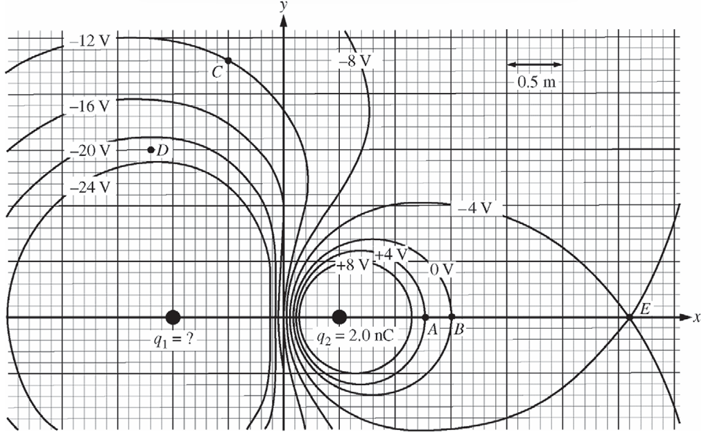
Using the \(0\text{ V}\) line intersection on the \(x\)-axis between the two charges at \(x = +0.20\text{ m}\):
The distance from \(q_{1}\) (at \(x = -1.00\text{ m}\)) to this point is \(r_{1} = 1.20\text{ m}\).
The distance from \(q_{2}\) (at \(x = +0.50\text{ m}\)) to this point is \(r_{2} = 0.30\text{ m}\).
Setting the net potential to zero:
\(V = \dfrac{k q_{1}}{r_{1}} + \dfrac{k q_{2}}{r_{2}} = 0\)
\(\dfrac{q_{1}}{1.20\text{ m}} = -\dfrac{2.0\text{ nC}}{0.30\text{ m}}\)
\(q_{1} = -4 \times 2.0\text{ nC} = -8.0\text{ nC}\)
Alternatively, using point \(B\) where \(V = 0\text{ V}\) at \(x = +1.00\text{ m}\) as shown in the scoring parameters:
\(r_{1} = 2.00\text{ m}\) and \(r_{2} = 0.50\text{ m}\)
\(\dfrac{k q_{1}}{2.0\text{ m}} + \dfrac{k q_{2}}{0.5\text{ m}} = 0\)
\(\boxed{q_{1} = -5.0\text{ nC}}\)

(b)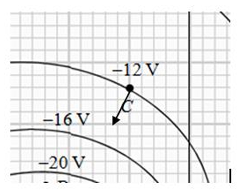

Electric field lines point in the direction of decreasing electric potential and must always remain locally perpendicular to equipotential boundaries.
At point \(C\), the vector should point perpendicularly away from the \(-12\text{ V}\) surface and point directly towards the next lower potential line, which is the \(-16\text{ V}\) contour line.
\(\boxed{\text{Vector drawn perpendicular to the line at C, pointing down and slightly left towards the }-16\text{ V line}}\)

(c)
The magnitude of the component of the electric field is estimated by the rate of change of potential over distance:
\(|E| \approx \left| \dfrac{\Delta V}{\Delta x} \right|\)
From the grid layout near point \(D\), the potential drops from \(-20\text{ V}\) to \(-24\text{ V}\) over a distance of approximately \(2\) grid squares (\(\Delta x \approx 2 \times 0.1\text{ m} = 0.2\text{ m}\)):
\(E = \dfrac{-20\text{ V} – (-24\text{ V})}{0.2\text{ m}} = 20\text{ V/m}\)
\(\boxed{E = 20\text{ N/C}\text{ (or }\text{V/m)}}\)

(d)
Applying Gauss’s law, the net electric flux leaving any closed boundary matches the enclosed target charge divided by the permittivity constant:
\(\Phi_{E} = \oint \vec{E} \cdot d\vec{A} = \dfrac{Q_{\text{enc}}}{\varepsilon_{0}}\)
The nearly spherical \(0\text{ V}\) boundary completely surrounds only the positive point charge \(q_{2} = +2.0\text{ nC}\):
\(\Phi_{E} = \dfrac{2.0 \times 10^{-9}\text{ C}}{8.85 \times 10^{-12}\text{ C}^{2}/(\text{N}\cdot\text{m}^{2})}\)
\(\Phi_{E} = 226\text{ N}\cdot\text{m}^{2}/\text{C}\)
\(\boxed{\Phi_{E} = 226\text{ N}\cdot\text{m}^{2}/\text{C}}\)

(e) i.
The conservative work executed by an electrostatic field distribution corresponds to the negative of its shifting potential energy status:
\(W = -q \Delta V = -q (V_{E} – V_{A})\)
From the chart coordinates, Point \(A\) rests precisely on the \(+4\text{ V}\) line, while Point \(E\) marks the intersection on the \(-4\text{ V}\) line:
\(W = -(1.60 \times 10^{-19}\text{ C})(-4\text{ V} – 4\text{ V})\)
\(W = -(1.60 \times 10^{-19}\text{ C})(-8\text{ V}) = 1.28 \times 10^{-18}\text{ J}\)
\(\boxed{W = 1.28 \times 10^{-18}\text{ J}\text{ (or }8.0\text{ eV)}}\)

(e) ii.
By the work-energy theorem, the kinetic energy gained matches the net work performed by the electric field:
\(W = \Delta K = \dfrac{1}{2} m v^{2}\)
Substituting the mass of a proton (\(m_{p} = 1.67 \times 10^{-27}\text{ kg}\)):
\(1.28 \times 10^{-18}\text{ J} = \dfrac{1}{2} (1.67 \times 10^{-27}\text{ kg}) v^{2}\)
\(v^{2} = \dfrac{2 \times 1.28 \times 10^{-18}\text{ J}}{1.67 \times 10^{-27}\text{ kg}}\)
\(v = \sqrt{1.533 \times 10^{9}} \approx 3.92 \times 10^{4}\text{ m/s}\)
\(\boxed{v = 3.92 \times 10^{4}\text{ m/s}}\)

(f)
Correct Selection: Left

Justification:
Electric field lines point perpendicularly away from equipotential contours and toward lower electric potential values, meaning the electric field vector at point \(B\) points to the right.
Because an electron possesses a negative fundamental charge, the mechanical electric force it experiences acts in a direction directly opposite to the local electric field vector.
Consequently, following Newton’s second law \( \vec{a} = \dfrac{\vec{F}}{m} \), the electron’s initial acceleration will be directed toward the left.