
AP Physics C- E&M- 9.1 Electric Potential Energy- Exam Style questions - FRQs- New Syllabus
Question

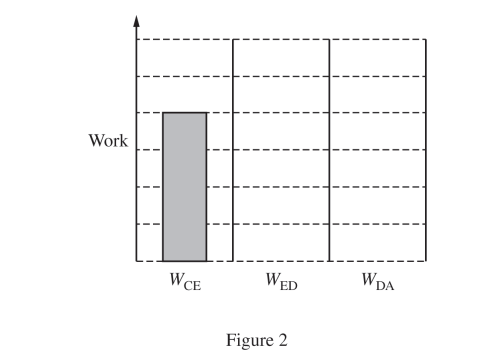
• Draw a bar to represent the relative absolute value of the work \(W_{ED}\) done by the external force on the test charge to move the test charge from Position \(E\) to Position \(D\).
• Draw a bar to represent the relative absolute value of the work \(W_{DA}\) done by the external force on the test charge to move the test charge from Position \(D\) to Position \(A\).
• The height of each bar should be proportional to the value of \(W_{CE}\). If \(W_{ED}=0\) and/or \(W_{DA}=0\), write \(0\) in the corresponding column, as appropriate.

_____ \(-x\) _____ \(-y\) _____ Directly toward the sphere

Most-appropriate topic codes (AP Physics C: Electricity and Magnetism):
• Topic \(8.6\) — Gauss’s Law (Part \( \mathrm{a} \))
• Topic \(9.1\) — Electric Potential Energy (Part \( \mathrm{b(i)} \))
• Topic \(9.2\) — Electric Potential (Parts \( \mathrm{b} \), \( \mathrm{c} \), \( \mathrm{d} \))
• Topic \(8.3\) — Electric Fields (Parts \( \mathrm{b(ii)} \), \( \mathrm{c} \), \( \mathrm{d(ii)} \))
• Topic \(8.4\) — Electric Fields of Charge Distributions (Part \( \mathrm{d} \))
▶️ Answer/Explanation
(a)
Use Gauss’s law:
\( \Phi_E=\dfrac{Q_{\text{enc}}}{\varepsilon_0} \)
The \(0.0\,\text{V}\) equipotential surface encloses the sphere with charge \(+1.0\,\text{nC}\). Therefore,
\( \left|\Phi_E\right|=\left|\dfrac{1.0\times 10^{-9}\,\text{C}}{8.85\times 10^{-12}\,\text{C}^2/(\text{N}\cdot\text{m}^2)}\right| \)
\( \boxed{\left|\Phi_E\right|=113\,\text{N}\cdot\text{m}^2/\text{C}} \)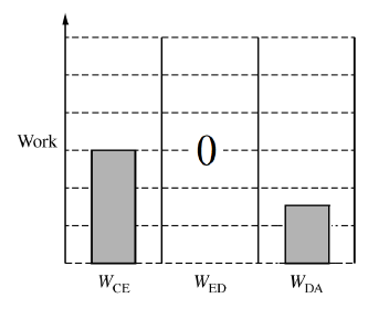
(b)(i)
For a test charge moved slowly by an external force, the work done by the external force is related to the change in electric potential energy:
\( W_{\text{ext}}=\Delta U=q\Delta V \)
Since the test charge is positive, the absolute value of the work is proportional to the absolute value of the potential difference:
\( |W_{\text{ext}}|\propto |\Delta V| \)
From the equipotential diagram, \(E\) and \(D\) are on the same \(0.0\,\text{V}\) equipotential line, so
\( \boxed{W_{ED}=0} \)
The potential difference from \(D\) to \(A\) is larger than the potential difference from \(C\) to \(E\). Specifically, \(W_{DA}\) should be represented by a bar approximately \(1.5\) times the height of the \(W_{CE}\) bar.
\( \boxed{W_{DA}\approx 1.5W_{CE}} \)
(b)(ii)
The electric field component can be estimated from the potential difference between nearby equipotential lines:
\( E_x=-\dfrac{\Delta V}{\Delta x} \)
Near Position \(B\), the relevant equipotential values are approximately \(-10.0\,\text{V}\) and \(-20.0\,\text{V}\), separated by about \(1.4\,\text{m}\).
\( |E_x|\approx \left|\dfrac{-20.0\,\text{V}-(-10.0\,\text{V})}{1.4\,\text{m}}\right| \)
\( |E_x|\approx \dfrac{10.0\,\text{V}}{1.4\,\text{m}} \)
\( \boxed{|E_x|\approx 7.1\,\text{V/m}} \)
(c)
Correct direction:
\( \boxed{-y} \)
The electric field is always perpendicular to equipotential lines and points in the direction of decreasing electric potential. Since the test charge is positive, the electric force on it is in the same direction as the electric field. At Position \(C\), the direction of decreasing potential is downward, so the net electric force is in the \(-y\)-direction.
(d)(i)
Treat the rod as a collection of small charge elements. Let a small element of the rod have length \(dy\), so
\( dq=-\lambda\,dy \)
The distance from this charge element at position \(y\) to point \(P\) is
\( r=y_P-y \)
The contribution to the electric potential is
\( dV=\dfrac{k\,dq}{r} \)
Substitute \(dq=-\lambda\,dy\):
\( dV=\dfrac{k(-\lambda\,dy)}{y_P-y} \)
\( V_P=-k\lambda\int_{0}^{2L}\dfrac{1}{y_P-y}\,dy \)
Evaluate the integral:
\( \int\dfrac{1}{y_P-y}\,dy=-\ln(y_P-y) \)
Therefore,
\( V_P=-k\lambda\left[-\ln(y_P-y)\right]_{0}^{2L} \)
\( V_P=-k\lambda\left[-\ln(y_P-2L)+\ln(y_P)\right] \)
\( V_P=-k\lambda\ln\left(\dfrac{y_P}{y_P-2L}\right) \)
\( \boxed{V_P=-k\lambda\ln\left(\dfrac{y_P}{y_P-2L}\right)} \)
(d)(ii)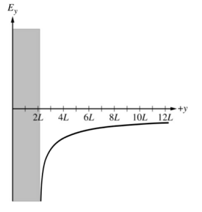
The \(y\)-component of the electric field can be found from the potential:
\( E_y=-\dfrac{dV}{dy} \)
Since the rod is negatively charged, the electric field above the rod points downward, toward the rod. Therefore, for \(y>2L\),
\( E_y<0 \)
The magnitude is very large near \(y=2L\), then decreases as \(y\) becomes larger. Thus the graph should be entirely below the horizontal axis, concave down, and should approach \(0\) from below as \(y\) increases.
A mathematical form consistent with this shape is
\( E_y=-\dfrac{2k\lambda L}{y(y-2L)} \)
so the curve is negative for \(2L<y<12L\) and approaches \(0\) as \(y\) increases.