
AP Physics C Mechanics - 5.1 Rotational Kinematics- Exam Style questions- FRQs
Rotational Kinematics AP Physics C Mechanics FRQ
Unit 5: Torque and Rotational Dynamics
Weightage : 10-15%
Question
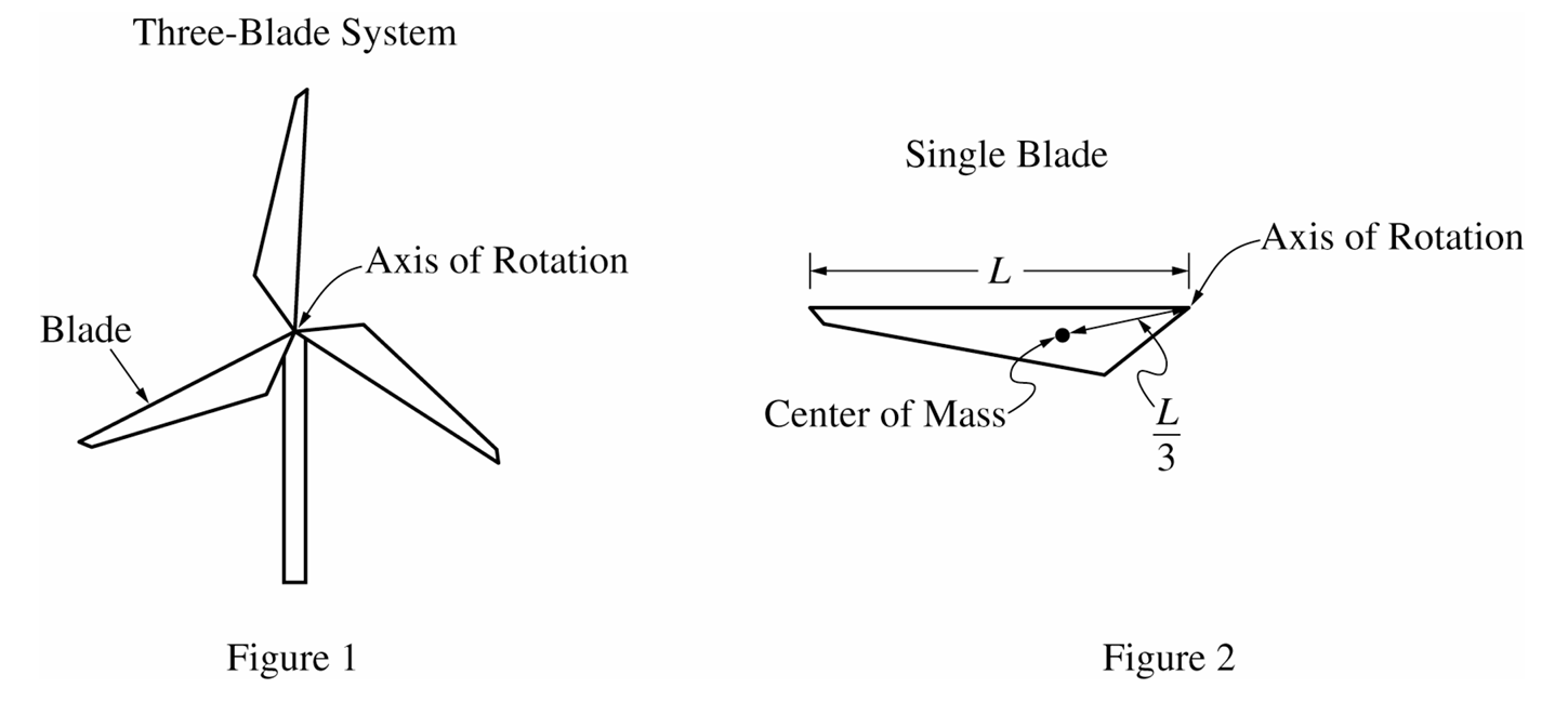
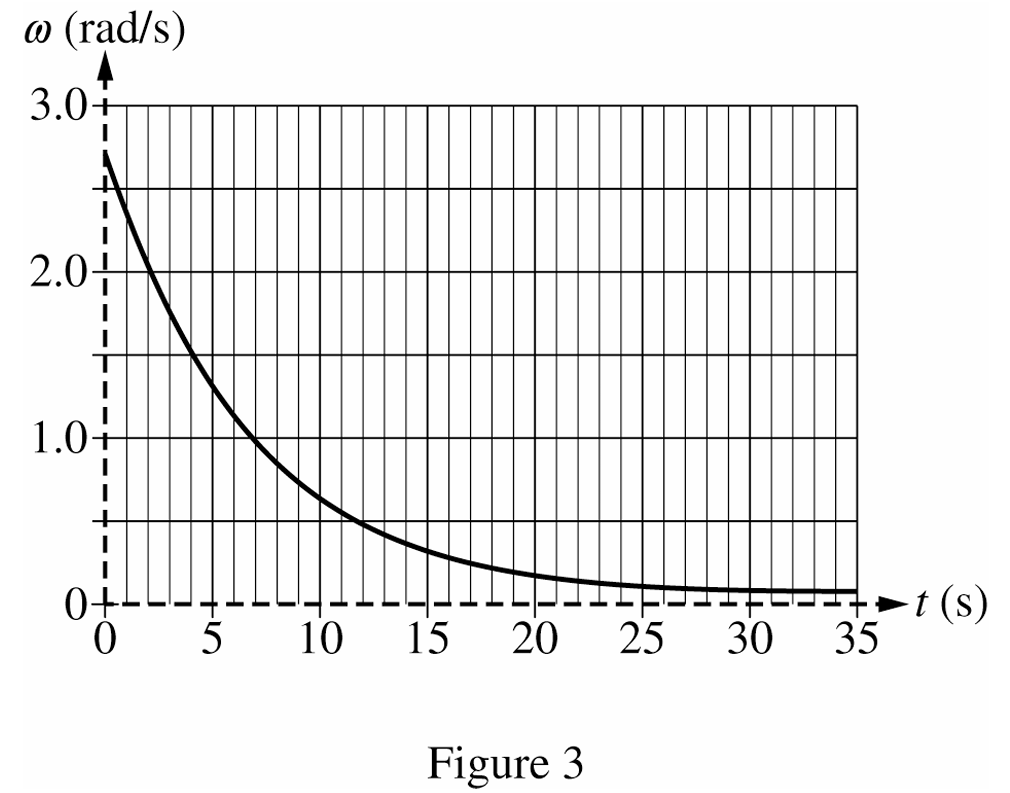
ii. Derive an expression for the net torque exerted on the system as a function of \(t\) as the system slows down. Express your answers in terms of \(\beta_0\), \(\omega_0\), \(M\), \(L\), \(I_{sys}\), and physical constants, as appropriate.
iii. Derive an expression for the angular displacement of the system \(\Delta\theta\) as a function of \(t\). Express your answer in terms of \(\beta_0\), \(\omega_0\), \(M\), \(L\), \(I_{sys}\), and physical constants, as appropriate.
Most-appropriate topic codes (AP Physics C: Mechanics):
• Topic \(5.1\) — Rotational Kinematics (Parts \( \mathrm{b} \), \( \mathrm{c(iii)} \), \( \mathrm{d} \))
• Topic \(6.1\) — Rotational Kinetic Energy (Part \( \mathrm{c(i)} \))
• Topic \(5.6\) — Newton’s Second Law in Rotational Form (Part \( \mathrm{c(ii)} \))
▶️ Answer/Explanation
(a)
Use the parallel-axis theorem to find the rotational inertia of one blade about the rotation axis:
\( I_{\text{blade}}=I_{CM}+Md^2 \)
\( I_{\text{blade}}=\dfrac{1}{18}ML^2+M\left(\dfrac{L}{3}\right)^2 \)
\( I_{\text{blade}}=\dfrac{1}{18}ML^2+\dfrac{1}{9}ML^2=\dfrac{1}{6}ML^2 \)
Multiply the rotational inertia of one blade by \(3\) to get the total rotational inertia:
\( I_{\text{rotor}}=3I_{\text{blade}}=3\left(\dfrac{1}{6}ML^2\right) \)
\( \boxed{I_{\text{rotor}}=\dfrac{1}{2}ML^2} \)
(b)
The time to complete one revolution is the period \(T\):
\( \omega_0=\dfrac{2\pi}{T} \)
\( T=\dfrac{2\pi}{\omega_0} \)
\( T=\dfrac{2\pi}{2.6\,\text{rad/s}} \)
\( \boxed{T=2.4\,\text{s}} \)
(c)(i)
The amount of energy dissipated is equal to the total initial rotational kinetic energy:
\( E_{\text{dis}}=\Delta K_{\text{rot}} \)
\( E_{\text{dis}}=0-\dfrac{1}{2}I_{sys}\omega_0^2 \)
\( E_{\text{dis}}=-\dfrac{1}{2}(6.7\times 10^6\,\text{kg}\cdot\text{m}^2)(2.6\,\text{rad/s})^2 \)
\( \boxed{E_{\text{dis}}=-2.3\times 10^7\,\text{J}} \)
(c)(ii)
Apply Newton’s second law in rotational form:
\( \tau=I_{sys}\alpha \)
\( \tau=I_{sys}\dfrac{d\omega}{dt} \)
\( \tau=I_{sys}\dfrac{d}{dt}\left(\omega_0e^{-\beta_0t}\right) \)
\( \boxed{\tau=-\beta_0I_{sys}\omega_0e^{-\beta_0t}} \)
(c)(iii)
Integrate the expression for angular speed to find angular displacement:
\( \Delta\theta=\int_0^t \omega(t)\,dt \)
\( \Delta\theta=\int_0^t \omega_0e^{-\beta_0t}\,dt \)
\( \Delta\theta=\left[-\dfrac{\omega_0}{\beta_0}e^{-\beta_0t}\right]_0^t \)
\( \Delta\theta=-\dfrac{\omega_0}{\beta_0}e^{-\beta_0t}-\left(-\dfrac{\omega_0}{\beta_0}(1)\right) \)
\( \boxed{\Delta\theta=\dfrac{\omega_0}{\beta_0}\left(1-e^{-\beta_0t}\right)} \)
(d)
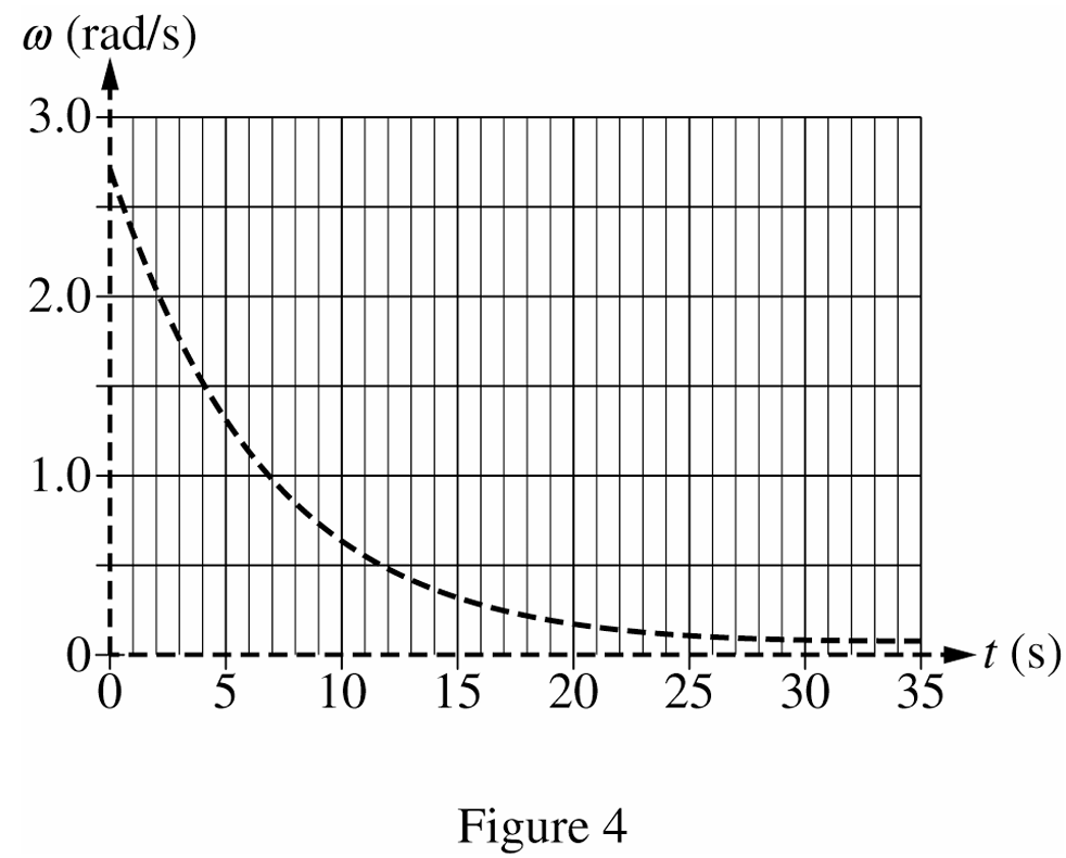
Draw a continuous curve showing an exponential decay. Because \(\beta>\beta_0\), the new system slows down faster. The new curve must start at the same initial angular speed, \(\omega_0=2.6\,\text{rad/s}\), and decay entirely below the original dashed curve.