
AP Physics C Mechanics - 3.2 Work- Exam Style questions- FRQs
Work AP Physics C Mechanics FRQ
Unit 3: Work, Energy, and Power
Weightage : 15-25%
Question
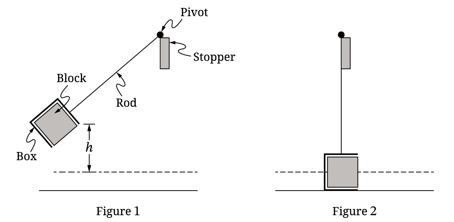
Describe an experimental procedure using the described setup to collect data that would allow the students to determine an experimental value of \(g\) using a linear graph. Include any steps necessary to reduce experimental uncertainty.
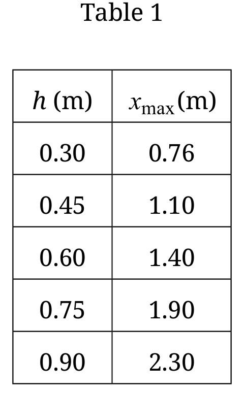
i. Indicate two quantities, either measured quantities from Table 1 or additional calculated quantities, that could be graphed to produce a straight line that could be used to determine \(\mu\).
Vertical axis: _____________ Horizontal axis: _____________
ii. On the grid provided, create a graph of the quantities indicated in part C (i).
- Use Table 2 to record the measured or calculated quantities that you will plot.
- Clearly label the axes, including units as appropriate.
- Plot the points you recorded in Table 2.

Most-appropriate topic codes (AP Physics C: Mechanics):
• Topic \(2.7\) — Kinetic and Static Friction (Parts C, D)
• Topic \(3.2\) — Work (Parts C, D)
▶️ Answer/Explanation
(A)
Measure the height \(h\) at which the block-box system is released using the meterstick. Release the system from rest. Measure the speed \(v\) of the block as it slides across the horizontal surface using the motion sensor. Repeat the measurement of the speed multiple times for the same release height \(h\) to reduce experimental uncertainty, and repeat the experiment for various release heights.
(B)
Plot \(v^2\) on the vertical axis and \(2h\) on the horizontal axis.
According to the conservation of energy, the gravitational potential energy transforms into kinetic energy:
\(mgh = \frac{1}{2}mv^2 \Rightarrow v^2 = 2gh\)
The slope of the best-fit line of \(v^2\) vs. \(2h\) will yield a straight line whose slope is directly equal to \(g\).
(C)(i)
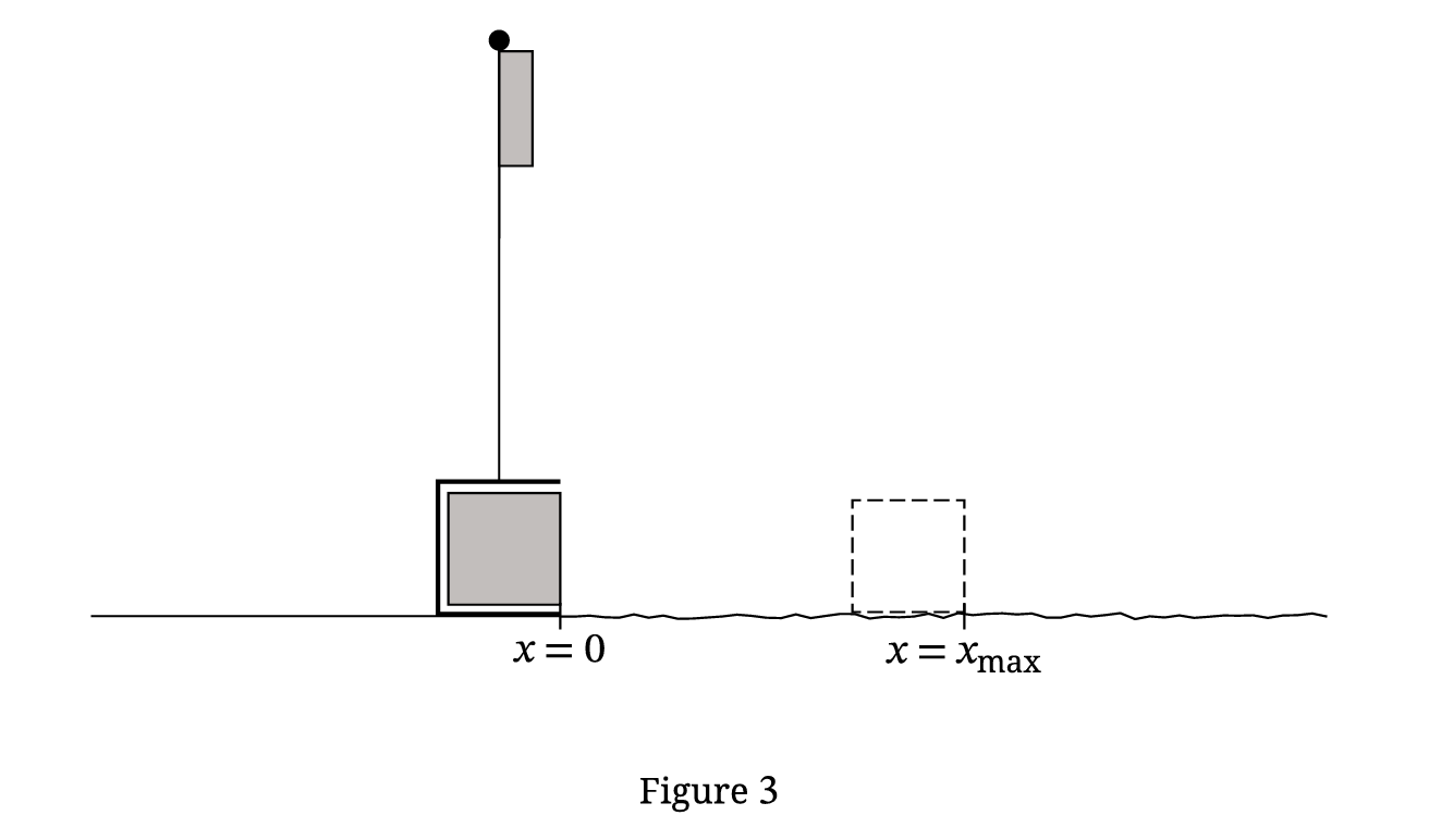
Applying the work-energy theorem to the entire path, the initial potential energy is dissipated by the work done by kinetic friction:
\(mgh – \mu mg x_{max} = 0 \Rightarrow h = \mu x_{max}\)
Therefore, to determine \(\mu\), we can graph \(h\) on the vertical axis and \(x_{max}\) on the horizontal axis.
(C)(ii)
The vertical axis should be correctly labeled as \(h\) with units \((\text{m})\) and a linear scale, and the horizontal axis should be correctly labeled as \(x_{max}\) with units \((\text{m})\) and a linear scale. The data points from Table 1 are accurately plotted on the grid according to these axes.
(C)(iii)
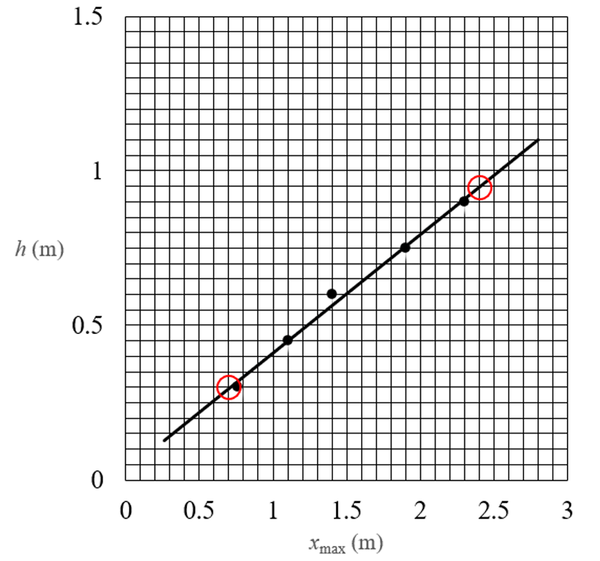
A straight best-fit line is drawn that properly approximates the overall linear trend of the plotted data points.
(D)
Based on the relationship \(h = \mu x_{max}\), the equation matches the linear form \(y = mx + b\) with a \(y\)-intercept of \(0\). The slope of the best-fit line is equal to \(\mu\).
Selecting two arbitrary points on the drawn best-fit line to calculate the slope, for example, \((0.70\,\text{m}, 0.30\,\text{m})\) and \((2.4\,\text{m}, 0.95\,\text{m})\):
\(\text{Slope} = \dfrac{\Delta h}{\Delta x_{max}}\)
\(\text{Slope} = \dfrac{0.95 – 0.30}{2.4 – 0.70}\)
\(\text{Slope} = 0.38\)
\(\mu = 0.38\)