Rewriting Polynomial and Rational Expressions (Factored Form)
Writing polynomial and rational expressions in factored form is especially useful because it clearly reveals important features of a function.
In factored form, a polynomial or rational function is written as a product of factors, rather than as a sum of terms.
For a polynomial function, the factored form looks like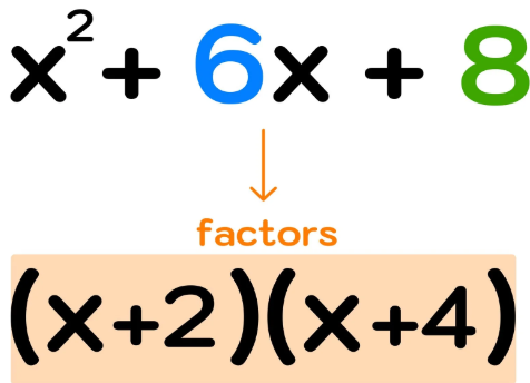
\( \mathrm{ f(x) = a(x – r_1)(x – r_2)\dots(x – r_n) } \)
For a rational function, the factored form looks like
\( \mathrm{ r(x) = \dfrac{(x – a_1)(x – a_2)\dots}{(x – b_1)(x – b_2)\dots} } \)
Why Factored Form Is Important
• Real zeros and x-intercepts are found by setting each factor equal to zero
• Factors in the denominator show where the function is undefined
• Common factors in the numerator and denominator indicate holes
• Remaining denominator factors indicate vertical asymptotes
Because of this, factored form is the best form for analyzing intercepts, holes, and asymptotes.
Example :
Rewrite the polynomial in factored form and identify its real zeros:
\( \mathrm{ f(x) = x^2 – 7x + 10 } \)
▶️ Answer/Explanation
Factor the quadratic:
\( \mathrm{ f(x) = (x – 5)(x – 2) } \)
Set each factor equal to zero:
\( \mathrm{ x – 5 = 0 \Rightarrow x = 5 } \)
\( \mathrm{ x – 2 = 0 \Rightarrow x = 2 } \)
Conclusion
The real zeros are \( \mathrm{x = 2} \) and \( \mathrm{x = 5} \), which are the x-intercepts.
Example :
Rewrite the rational expression in factored form and identify any holes or vertical asymptotes:
\( \mathrm{ r(x) = \dfrac{x^2 – 9}{x^2 – 3x} } \)
▶️ Answer/Explanation
Factor the numerator and denominator:
\( \mathrm{ x^2 – 9 = (x – 3)(x + 3) } \)
\( \mathrm{ x^2 – 3x = x(x – 3) } \)
Cancel the common factor \( \mathrm{(x – 3)} \):
\( \mathrm{ r(x) = \dfrac{x + 3}{x},\; x \ne 3 } \)
Interpretation
There is a hole at \( \mathrm{x = 3} \).
There is a vertical asymptote at \( \mathrm{x = 0} \).
Rewriting Polynomial and Rational Expressions (Standard Form)
Writing polynomial and rational expressions in standard form highlights the overall structure of a function and is especially useful for analyzing end behavior.
In standard form, terms are written in descending powers of the variable.
Standard Form of a Polynomial
\( \mathrm{ f(x) = a_n x^n + a_{n-1} x^{n-1} + \dots + a_1 x + a_0 } \)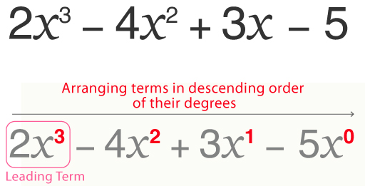
In this form:
• The degree of the polynomial is \( \mathrm{n} \)
• The leading term is \( \mathrm{a_n x^n} \)
• The leading coefficient is \( \mathrm{a_n} \)
The leading term determines the end behavior of the graph.
Standard Form of a Rational Function
A rational function written in standard form is
\( \mathrm{ r(x) = \dfrac{p(x)}{q(x)} } \)
where both \( \mathrm{p(x)} \) and \( \mathrm{q(x)} \) are written in standard polynomial form.
Standard form is useful for:
• Identifying degrees of numerator and denominator
• Determining horizontal or slant asymptotes
• Describing long-term behavior of the function
Example :
Rewrite the polynomial in standard form and describe its end behavior:
\( \mathrm{ f(x) = 3 – 2x^3 + x^2 } \)
▶️ Answer/Explanation
Standard form
\( \mathrm{ f(x) = -2x^3 + x^2 + 3 } \)
The leading term is \( \mathrm{-2x^3} \).
The degree is odd and the leading coefficient is negative.
Conclusion
As \( \mathrm{x \to \infty} \), \( \mathrm{f(x) \to -\infty} \), and as \( \mathrm{x \to -\infty} \), \( \mathrm{f(x) \to \infty} \).
Example :
Rewrite the rational function in standard form and determine its end behavior:
\( \mathrm{ r(x) = \dfrac{4x – 1 + x^2}{2 – x^2} } \)
▶️ Answer/Explanation
Standard form
\( \mathrm{ r(x) = \dfrac{x^2 + 4x – 1}{-x^2 + 2} } \)
Both numerator and denominator have degree 2.
The quotient of leading coefficients is
\( \mathrm{ \dfrac{1}{-1} = -1 } \)
Conclusion
The graph has a horizontal asymptote at \( \mathrm{y = -1} \).
Polynomial Long Division
Polynomial long division is an algebraic process that is analogous to numerical long division.
It is used to divide one polynomial by another polynomial, resulting in a quotient and a remainder.
If a polynomial \( \mathrm{f(x)} \) is divided by a polynomial \( \mathrm{g(x)} \), then \( \mathrm{f(x)} \) can be rewritten as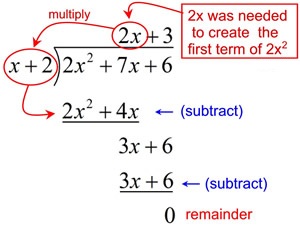
\( \mathrm{ \displaystyle f(x) = g(x)\,q(x) + r(x) } \)
where:
• \( \mathrm{q(x)} \) is the quotient
• \( \mathrm{r(x)} \) is the remainder
• The degree of \( \mathrm{r(x)} \) is less than the degree of \( \mathrm{g(x)} \)
Polynomial long division is especially useful for rewriting rational functions, identifying slant asymptotes, and expressing functions in equivalent forms.
Example :
Divide
\( \mathrm{ \displaystyle f(x) = x^3 – 4x^2 + x + 6 } \)
by
\( \mathrm{ \displaystyle g(x) = x – 2 } \)
▶️ Answer/Explanation
Perform polynomial long division.
The quotient is
\( \mathrm{ \displaystyle q(x) = x^2 – 2x – 3 } \)
The remainder is
\( \mathrm{ \displaystyle r(x) = 0 } \)
Rewrite the function
\( \mathrm{ \displaystyle f(x) = (x – 2)(x^2 – 2x – 3) } \)
Since the remainder is zero, the division is exact.
Example :
Divide
\( \mathrm{ \displaystyle f(x) = 2x^3 + x^2 – 5x + 1 } \)
by
\( \mathrm{ \displaystyle g(x) = x + 1 } \)
▶️ Answer/Explanation
After performing polynomial long division:
The quotient is
\( \mathrm{ \displaystyle q(x) = 2x^2 – x – 4 } \)
The remainder is
\( \mathrm{ \displaystyle r(x) = 5 } \)
Rewrite the function
\( \mathrm{ \displaystyle f(x) = (x + 1)(2x^2 – x – 4) + 5 } \)
The remainder has degree 0, which is less than the degree of \( \mathrm{g(x)} \).
Using Polynomial Long Division to Find Slant Asymptotes
Polynomial long division is especially useful when analyzing the graphs of rational functions.
When the degree of the polynomial in the numerator is exactly one greater than the degree of the polynomial in the denominator, the graph of the rational function has a slant asymptote.
Performing polynomial long division rewrites the rational function in the form
\( \mathrm{ \displaystyle r(x) = q(x) + \dfrac{r(x)}{g(x)} } \)
As the input values increase or decrease without bound, the fraction involving the remainder approaches zero.
Therefore, the graph of the rational function approaches the graph of the quotient polynomial.
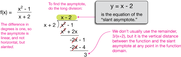
If the quotient is a linear function, its equation gives the equation of the slant asymptote.
Example :
Find the slant asymptote of the rational function
\( \mathrm{ \displaystyle r(x) = \dfrac{x^2 + 3x + 1}{x + 1} } \)
▶️ Answer/Explanation
Perform polynomial long division:
\( \mathrm{ \displaystyle \dfrac{x^2 + 3x + 1}{x + 1} = x + 2 – \dfrac{1}{x + 1} } \)
As \( \mathrm{x \to \pm\infty} \), the fraction approaches 0.
Conclusion
The graph approaches the line
\( \mathrm{ \displaystyle y = x + 2 } \)
So the slant asymptote is \( \mathrm{y = x + 2} \).
Example :
Determine whether the rational function has a slant asymptote:
\( \mathrm{ \displaystyle f(x) = \dfrac{2x^3 – x}{x^2 + 1} } \)
▶️ Answer/Explanation
The degree of the numerator is one greater than the degree of the denominator.
Perform polynomial long division:
\( \mathrm{ \displaystyle \dfrac{2x^3 – x}{x^2 + 1} = 2x – \dfrac{3x}{x^2 + 1} } \)
The remainder term approaches 0 as \( \mathrm{x \to \pm\infty} \).
Conclusion
The graph approaches the line
\( \mathrm{ \displaystyle y = 2x } \)
So the rational function has a slant asymptote \( \mathrm{y = 2x} \).
The Binomial Theorem
The Binomial Theorem provides an efficient way to expand expressions of the form \( \mathrm{(a + b)^n} \), where \( \mathrm{n} \) is a nonnegative integer.
The coefficients in the expansion come from a single row of Pascal’s Triangle.
Using the Binomial Theorem, the expansion is given by
\( \mathrm{ \displaystyle (a + b)^n = \sum_{k=0}^{n} \binom{n}{k} a^{\,n-k} b^{\,k} } \)
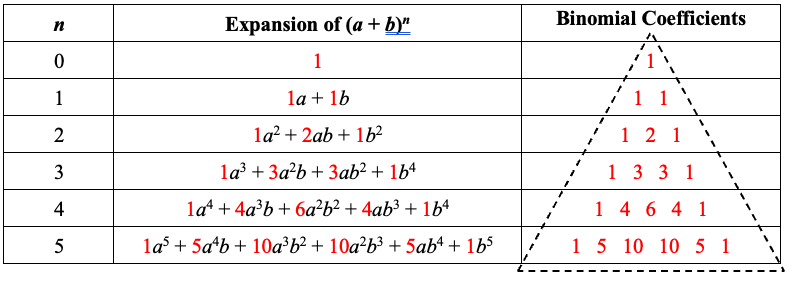
Here, \( \mathrm{\binom{n}{k}} \) represents the binomial coefficients, which match the entries in the \( \mathrm{n^{th}} \) row of Pascal’s Triangle.
This theorem is especially useful for expanding polynomial functions of the form
\( \mathrm{ \displaystyle p(x) = (x + c)^n } \)
where \( \mathrm{c} \) is a constant. The result is a polynomial written in standard form.
Example:
Use the Binomial Theorem to expand
\( \mathrm{ \displaystyle (x + 2)^3 } \)
▶️ Answer/Explanation
The coefficients from Pascal’s Triangle for \( \mathrm{n = 3} \) are
\( \mathrm{ 1,\; 3,\; 3,\; 1 } \)
Apply the Binomial Theorem:
\( \mathrm{ \displaystyle (x + 2)^3 = x^3 + 3x^2(2) + 3x(2^2) + 2^3 } \)
Simplify:
\( \mathrm{ \displaystyle x^3 + 6x^2 + 12x + 8 } \)
Example:
Expand the polynomial function
\( \mathrm{ \displaystyle p(x) = (x – 1)^4 } \)
▶️ Answer/Explanation
The coefficients from Pascal’s Triangle for \( \mathrm{n = 4} \) are
\( \mathrm{ 1,\; 4,\; 6,\; 4,\; 1 } \)
Apply the Binomial Theorem:
\( \mathrm{ \displaystyle (x – 1)^4 = x^4 – 4x^3 + 6x^2 – 4x + 1 } \)
Conclusion
The Binomial Theorem allows this expansion to be completed quickly without repeated multiplication.