
▶️ Answer/Explanation
(A) (i)
First, evaluate the inner function \(f(5)\) using the table: \(f(5) = 34\).
Next, substitute this value into \(g(x)\) to find \(h(5) = g(34)\).
\(g(34) = \frac{34^3 – 14(34) – 27}{34 + 2}\)
\(g(34) = \frac{39304 – 476 – 27}{36} = \frac{38801}{36}\)
\(h(5) \approx 1077.806\)
(A) (ii)
To find \(f^{-1}(4)\), we look for the input value \(x\) in the table that produces an output of \(4\).
The table shows that \(f(3) = 4\).
Therefore, \(f^{-1}(4) = 3\).
(B) (i)
Set \(g(x) = 3\) and solve for \(x\):
\(\frac{x^3 – 14x – 27}{x + 2} = 3\)
Multiply both sides by \((x+2)\): \(x^3 – 14x – 27 = 3(x + 2)\)
Simplify: \(x^3 – 14x – 27 = 3x + 6\)
Rearrange into polynomial form: \(x^3 – 17x – 33 = 0\)
Using a graphing calculator to find the zero of this polynomial:
\(x \approx 4.879\)
(B) (ii)
We evaluate the limit as \(x \to -\infty\) for \(g(x)\).
\(\lim_{x \to -\infty} \frac{x^3 – 14x – 27}{x + 2}\)
By examining the leading terms, the function behaves like \(\frac{x^3}{x} = x^2\) for large absolute values of \(x\).
As \(x \to -\infty\), \(x^2 \to \infty\).
\(\lim_{x \to -\infty} g(x) = \infty\)
(C) (i)
Calculate the first differences of \(f(x)\): \((-5) – (-10) = 5\), \(4 – (-5) = 9\), \(17 – 4 = 13\), \(34 – 17 = 17\).
Calculate the second differences: \(9 – 5 = 4\), \(13 – 9 = 4\), \(17 – 13 = 4\).
Since the second differences are constant, \(f\) is best modeled by a quadratic function.
(C) (ii)
The model is quadratic because for equal intervals of the input values \(x\) (step size of \(1\)), the rate of change of the output values increases by a constant amount (constant second difference of \(4\)).
Question
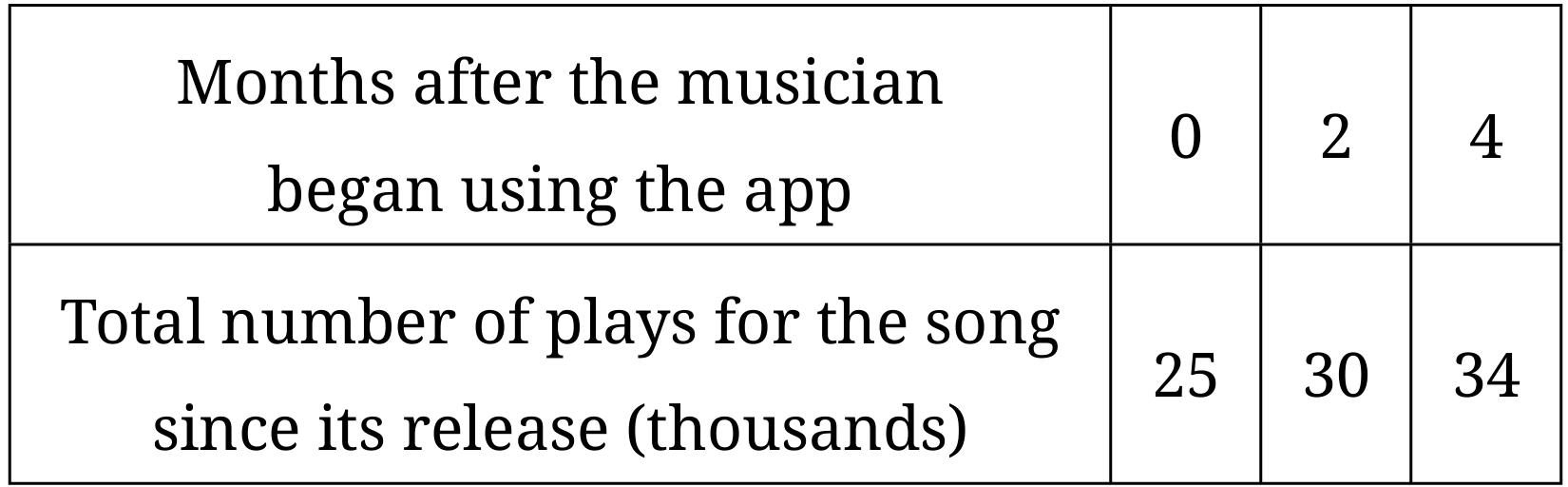
(i) Use the given data to write three equations that can be used to find the values for constants \( a \), \( b \), and \( c \) in the expression for \( D(t) \).
(ii) Find the values for \( a \), \( b \), and \( c \) as decimal approximations.
(i)Use the given data to find the average rate of change of the total number of plays for the song, in thousands per month, from \( t = 0 \) to \( t = 4 \) months. Express your answer as a decimal approximation. Show the computations that lead to your answer.
(ii) Use the average rate of change found in part B (i) to estimate the total number of plays for the song, in thousands, for \( t = 1.5 \) months. Show the work that leads to your answer.
(iii) Let \( A_t \) represent the estimate of the total number of plays for the song, in thousands, using the average rate of change found in part B (i). For \( A_{1.5} \) found in part B (ii), it can be shown that \( A_{1.5} < D(1.5) \). Explain why, in general, \( A_t < D(t) \) for all \( t \), where \( 0 < t < 4 \). Your explanation should include a reference to the graph of \( D \) and its relationship to \( A_t \).
Most-appropriate topic codes (AP Precalculus 2024):
• 1.2: Compare rates of change using average rates of change — part B(i)
• 2.5: Construct a model for situations involving proportional output values — part B(ii)
• 1.3: Determine the change in average rates of change for quadratic functions — part B(iii)
• 1.13: Articulate model assumptions and domain restrictions — part C
▶️ Answer/Explanation
A.
(i)
Because \( D(0) = 25 \), \( D(2) = 30 \), and \( D(4) = 34 \), the three equations are: \[ \begin{align*} a(0)^2 + b(0) + c &= 25 \\ a(2)^2 + b(2) + c &= 30 \\ a(4)^2 + b(4) + c &= 34 \end{align*} \] These simplify to: \[ \begin{align*} c &= 25 \quad \text{(1)} \\ 4a + 2b + c &= 30 \quad \text{(2)} \\ 16a + 4b + c &= 34 \quad \text{(3)} \end{align*} \] ✅ Answer: \(\boxed{c=25, \; 4a+2b+c=30, \; 16a+4b+c=34}\)
(ii)
Substitute \( c = 25 \) into (2) and (3): \[ \begin{align*} 4a + 2b &= 5 \quad \text{(2′)} \\ 16a + 4b &= 9 \quad \text{(3′)} \end{align*} \] Multiply (2′) by 2: \( 8a + 4b = 10 \).
Subtract this from (3′): \( (16a+4b) – (8a+4b) = 9 – 10 \) gives \( 8a = -1 \), so \( a = -\frac{1}{8} = -0.125 \).
Substitute into (2′): \( 4(-0.125) + 2b = 5 \) gives \( -0.5 + 2b = 5 \), so \( 2b = 5.5 \), \( b = 2.75 \).
✅ Answer: \(\boxed{a = -0.125, \; b = 2.75, \; c = 25}\)
Thus, \( D(t) = -0.125t^2 + 2.75t + 25 \).
B.
(i)
Average rate of change from \( t=0 \) to \( t=4 \): \[ \frac{D(4)-D(0)}{4-0} = \frac{34 – 25}{4} = \frac{9}{4} = 2.25 \] ✅ Answer: \(\boxed{2.25}\) thousand plays per month.
(ii)
Using the average rate of change, the linear estimate is \( A_t = D(0) + 2.25t = 25 + 2.25t \).
For \( t = 1.5 \): \[ A_{1.5} = 25 + 2.25(1.5) = 25 + 3.375 = 28.375 \] ✅ Answer: \(\boxed{28.375}\) thousand plays.
(iii)
The estimate \( A_t \) is the \( y \)-coordinate of a point on the secant line passing through \( (0, D(0)) \) and \( (4, D(4)) \).
Since \( D(t) \) is a quadratic with \( a = -0.125 < 0 \), its graph is concave down on \( 0 < t < 4 \).
For a concave-down function over an interval, the secant line connecting the endpoints lies below the graph of the function for all \( t \) in the open interval \( (0, 4) \).
Therefore, \( A_t < D(t) \) for all \( t \) where \( 0 < t < 4 \).
✅ Explanation: Concave-down shape places the secant line below the curve.
C.
The quadratic \( D(t) = -0.125t^2 + 2.75t + 25 \) has \( a < 0 \), so it has an absolute maximum (vertex).
Find vertex: \( t = -\frac{b}{2a} = -\frac{2.75}{2(-0.125)} = \frac{2.75}{0.25} = 11 \) months.
In the context, \( D(t) \) models the total number of plays since release, which cannot decrease. However, the quadratic model decreases after \( t = 11 \) (its maximum), which would imply the total plays go down—impossible in reality.
Therefore, the model is only valid up to the time it reaches its maximum. The domain of \( D \) should be restricted to \( t \le 11 \) months (or until the maximum is reached) to ensure the total plays are non-decreasing.
✅ Explanation: The absolute maximum at \( t = 11 \) gives a right endpoint for the domain because the total plays cannot decrease after that time.
▶️ Answer/Explanation
Part A
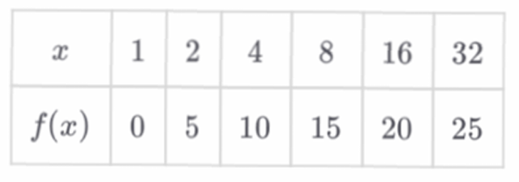
(i) From the table, we find $f(8) = 15$.
Substitute $15$ into the function $g(x)$: $h(8) = g(15) = 0.25(15)^3 – 9.5(15)^2 + 110(15) – 399$.
$h(8) = 0.25(3375) – 9.5(225) + 1650 – 399$.
$h(8) = 843.75 – 2137.5 + 1650 – 399$.
$h(8) = -42.75$.
(ii) To find $f^{-1}(20)$, we look for the $x$ value where $f(x) = 20$.
From the table, $f(16) = 20$.
Therefore, $f^{-1}(20) = 16$.
Part B
(i) We solve the equation $0.25x^3 – 9.5x^2 + 110x – 399 = -45$.
Set the equation to zero: $0.25x^3 – 9.5x^2 + 110x – 354 = 0$.
Using numerical methods or a graphing calculator, the real solutions are approximately:
$x \approx 5.242$
$x \approx 12.188$
$x \approx 20.570$
(ii) The end behavior of a polynomial is determined by its leading term, $0.25x^3$.
Since the leading coefficient is positive and the degree is odd, as $x \to \infty$, $g(x) \to \infty$.
The limit notation is $\lim_{x \to \infty} g(x) = \infty$.
Part C
(i) The function $f$ is best modeled by a logarithmic function.
(ii) In a logarithmic model, constant changes in the output values correspond to proportional changes in the input values.
As the output $f(x)$ increases by a constant $5$ ($0, 5, 10, 15 \dots$),
The input $x$ values are multiplied by a constant factor of $2$ ($1, 2, 4, 8 \dots$).
This constant ratio of inputs for constant additions of outputs is the hallmark of logarithmic growth.
▶️ Answer/Explanation
(A) (i)
First, evaluate the inner function \(f(5)\) using the table: \(f(5) = 34\).
Next, substitute this value into \(g(x)\) to find \(h(5) = g(34)\).
\(g(34) = \frac{34^3 – 14(34) – 27}{34 + 2}\)
\(g(34) = \frac{39304 – 476 – 27}{36} = \frac{38801}{36}\)
\(h(5) \approx 1077.806\)
(A) (ii)
To find \(f^{-1}(4)\), we look for the input value \(x\) in the table that produces an output of \(4\).
The table shows that \(f(3) = 4\).
Therefore, \(f^{-1}(4) = 3\).
(B) (i)
Set \(g(x) = 3\) and solve for \(x\):
\(\frac{x^3 – 14x – 27}{x + 2} = 3\)
Multiply both sides by \((x+2)\): \(x^3 – 14x – 27 = 3(x + 2)\)
Simplify: \(x^3 – 14x – 27 = 3x + 6\)
Rearrange into polynomial form: \(x^3 – 17x – 33 = 0\)
Using a graphing calculator to find the zero of this polynomial:
\(x \approx 4.879\)
(B) (ii)
We evaluate the limit as \(x \to -\infty\) for \(g(x)\).
\(\lim_{x \to -\infty} \frac{x^3 – 14x – 27}{x + 2}\)
By examining the leading terms, the function behaves like \(\frac{x^3}{x} = x^2\) for large absolute values of \(x\).
As \(x \to -\infty\), \(x^2 \to \infty\).
\(\lim_{x \to -\infty} g(x) = \infty\)
(C) (i)
Calculate the first differences of \(f(x)\): \((-5) – (-10) = 5\), \(4 – (-5) = 9\), \(17 – 4 = 13\), \(34 – 17 = 17\).
Calculate the second differences: \(9 – 5 = 4\), \(13 – 9 = 4\), \(17 – 13 = 4\).
Since the second differences are constant, \(f\) is best modeled by a quadratic function.
(C) (ii)
The model is quadratic because for equal intervals of the input values \(x\) (step size of \(1\)), the rate of change of the output values increases by a constant amount (constant second difference of \(4\)).