AP Precalculus -1.13 Function Models: Selection and Assumptions- MCQ Exam Style Questions - Effective Fall 2023

AP Precalculus -1.13 Function Models: Selection and Assumptions- MCQ Exam Style Questions – Effective Fall 2023

AP Precalculus -1.13 Function Models: Selection and Assumptions- MCQ Exam Style Questions – AP Precalculus- per latest AP Precalculus Syllabus.

AP Precalculus – MCQ Exam Style Questions- All Topics

Question

Water is poured into an empty vase at a constant rate. A graph (not shown) models the depth of the water in the vase over time. The graph can be described as follows: the graph is always increasing; the first portion of the graph is clearly concave up; and the next portion of the graph has a fairly steady and steep increase. Which of the following vases is appropriate for the context described by the graph?

▶️ Answer/Explanation

Detailed solution

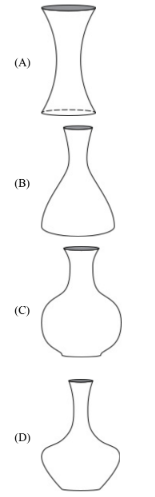
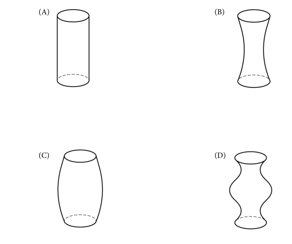
Water poured at constant rate → volume in vase increases linearly with time. Depth $ h $ vs. time $ t $ depends on horizontal cross-sectional area $ A(h) $: \[ \frac{dV}{dt} = \text{constant} \quad\text{and}\quad dV = A(h)\, dh \] so \[ \frac{dh}{dt} = \frac{\text{constant}}{A(h)}. \]

First portion concave up → $ \frac{dh}{dt} $ increasing with time → $ A(h) $ decreasing with $ h $. Thus bottom part of vase gets narrower as you go upward (like an upside-down cone or rounded bottom that narrows).

Next portion: fairly steady and steep increase → $ \frac{dh}{dt} $ nearly constant → $ A(h) $ constant → cylindrical section.

So correct vase shape: bottom part where cross-section narrows upward (giving concave up depth–time), then cylindrical section (giving linear depth–time = steep steady increase).

✅ Answer: (B)

Question

A music agent is planning a series of concerts at local farms around the nation. The agent is building a model to estimate crowd capacity based on different sizes of square fields. Which type of function is most likely to model crowd capacity in this situation?

(A) Linear
(B) Piecewise linear
(C) Quadratic
(D) Cubic

▶️ Answer/Explanation

Detailed solution

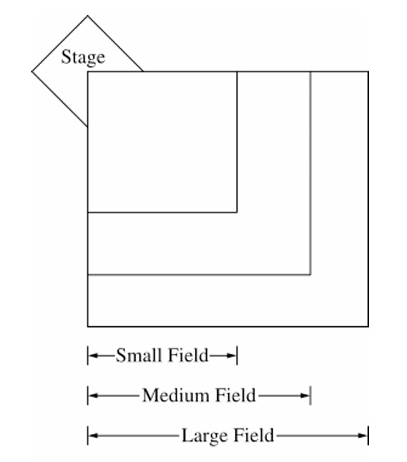
Capacity likely depends on the area of the square field. If side length = $ s $, then area = $ s^2 $, and crowd capacity is proportional to area (assuming constant density).
Thus capacity $ C(s) \propto s^2 $ ⇒ a quadratic function.
✅ Answer: (C)

Question

At a bakery, the number of cookies baked each day changes based on anticipated demand. The scatterplot shows the change in hundreds of cookies baked from the previous day for eight days. The point at (2, 5) means that on day 2, the number of cookies baked will be 500 more than the number of cookies baked on day 1. A function model $ C $ is to be constructed for the number of cookies baked on each of the days, 0 through 8. Which of the following statements best supports the selection of a model for $ C $?

(A) Because the information about rate of change is roughly linear, a linear model is best for $ C $.
(B) Because the information about rate of change is roughly linear, a quadratic model is best for $ C $.
(C) Because the information about rate of change is positive and negative, a quadratic model is best for $ C $.
(D) Because the information about rate of change is positive and negative, a piecewise-linear model is best for $ C $.

▶️ Answer/Explanation

Detailed solution

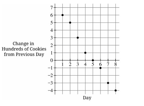
The given data is about change from previous day (i.e., daily increment in cookies baked).
If those daily increments (rate of change of total cookies baked) are roughly linear as a function of day number, that means the second differences of the total cookies are roughly constant ⇒ total cookies as a function of time is quadratic.
Thus: rate of change linear ⇒ total function quadratic.
✅ Answer: (B)

Question

The ancient Pythagoreans studied figurate numbers… The tetrahedral numbers are 1, 4, 10, 20, 35, 56, 84, etc. Which of the following statements is true?

(A) The tetrahedral numbers are best modeled by a quadratic function because the 2nd differences are a nonzero constant.
(B) The tetrahedral numbers are best modeled by a quadratic function because the 3rd differences are a nonzero constant.
(C) The tetrahedral numbers are best modeled by a cubic function because the 2nd differences are a nonzero constant.
(D) The tetrahedral numbers are best modeled by a cubic function because the 3rd differences are a nonzero constant.

▶️ Answer/Explanation

Detailed solution

Tetrahedral numbers formula is $ T_n = \frac{n(n+1)(n+2)}{6} $, a cubic polynomial in $ n $.
For a cubic polynomial, the third differences are constant and nonzero (while second differences are linear).
Thus correct reasoning: constant 3rd differences ⇒ cubic model.
✅ Answer: (D)

Question

At time $t=0$, water begins pouring into an empty container at a constant rate. The water pours into the container until it is full. The situation is modeled by the given graph (an S-curve where slope increases then decreases). For which of the following containers would the graph be appropriate?

▶️ Answer/Explanation

Detailed solution

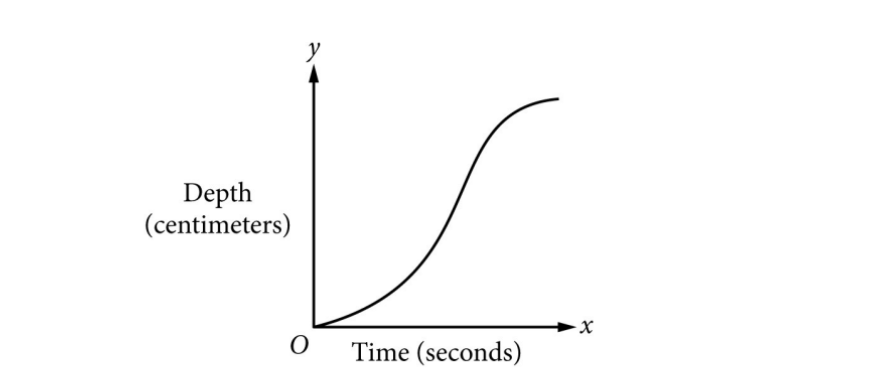
1. Relate Slope to Width:
Slope represents the rate of depth increase. A wide container fills slowly (small slope); a narrow container fills quickly (steep slope).

2. Analyze Graph Behavior:
The graph is concave up then concave down, meaning the slope starts low, increases to a maximum, then decreases. This implies: Wide $\rightarrow$ Narrow $\rightarrow$ Wide.

3. Match Container:
The hourglass shape fits this description (Wide bottom, narrow neck, wide top).

✅ Answer: (B)

Question

The table gives values for a function $g$ at selected values of $x$. Which of the following statements is true?

$x$	-1	0	1	2	3
$g(x)$	-3	-2	1	6	13

(A) $g$ is best modeled by a linear function…
(B) $g$ is best modeled by a quadratic function, because the average rates of change… are constant.
(C) $g$ is best modeled by a linear function…
(D) $g$ is best modeled by a quadratic function, because the successive 2nd differences of the output values over equal-interval input values are constant.

▶️ Answer/Explanation

Detailed solution

1. Calculate First Differences:
$-2 – (-3) = 1$
$1 – (-2) = 3$
$6 – 1 = 5$
$13 – 6 = 7$

2. Calculate Second Differences:
$3 – 1 = 2$
$5 – 3 = 2$
$7 – 5 = 2$

3. Conclusion:
Since second differences are constant, the function is quadratic.

✅ Answer: (D)

Question

The table shows the length of high-speed railways, in thousands of kilometers, in a certain country, starting in the year 2010 $(t=0)$. A quartic regression is used to model the length of high-speed railways as a function of years since 2010. What length of high-speed railways, in thousands of kilometers, is predicted by the model for 2028 $(t=18)$?

Year (time $t$)	2010 $(t=0)$	2013 $(t=3)$	2016 $(t=6)$	2019 $(t=9)$	2022 $(t=12)$
Length	1	7	16	25	38

(A) $54.2$
(B) $127.0$
(C) $309.3$
(D) $942.1$

▶️ Answer/Explanation

Detailed solution

1. Perform Quartic Regression:
Using a graphing calculator or statistical software, input the data points $(0,1), (3,7), (6,16), (9,25), (12,38)$ and select the Quartic Regression model ($y = ax^4 + bx^3 + cx^2 + dx + e$).
The resulting regression equation is approximately:
$L(t) \approx 0.00360t^4 – 0.08333t^3 + 0.68981t^2 + 0.58333t + 1$.

2. Predict for $t=18$ (Year 2028):
Substitute $t=18$ into the regression equation:
$L(18) \approx 0.00360(18)^4 – 0.08333(18)^3 + 0.68981(18)^2 + 0.58333(18) + 1$
Calculating the value yields approximately $127.0$.

✅ Answer: (B)

Question

The table shows values for a function $g$ at selected values of $x$. Which of the following claim and explanation statements best fits these data?

(A) $g$ is best modeled by a linear function, because the rate of change over consecutive equal-length input-value intervals is constant.
(B) $g$ is best modeled by a linear function, because the change in the average rates of change over consecutive equal-length input-value intervals is constant.
(C) $g$ is best modeled by a quadratic function, because the rate of change over consecutive equal-length input-value intervals is constant.
(D) $g$ is best modeled by a quadratic function, because the change in the average rates of change over consecutive equal-length input-value intervals is constant.

▶️ Answer/Explanation

Detailed solution

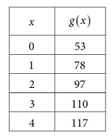
First compute average rates of change over intervals of length 1:
From $ x=0 $ to $ x=1 $: $ \frac{78-53}{1} = 25 $
From $ x=1 $ to $ x=2 $: $ \frac{97-78}{1} = 19 $
From $ x=2 $ to $ x=3 $: $ \frac{110-97}{1} = 13 $
From $ x=3 $ to $ x=4 $: $ \frac{117-110}{1} = 7 $

These rates are not constant, so not linear.
Now compute changes in these average rates (second differences):
$ 19 – 25 = -6 $
$ 13 – 19 = -6 $
$ 7 – 13 = -6 $
The change in average rates is constant ($-6$). This is characteristic of a quadratic function.
Thus $g$ is best modeled by a quadratic function because the change in average rates of change is constant.
✅ Answer: (D)

Question

The figure shows a portion of the graph of a function $f$. Which of the following conclusions is possible for $f$?

(A) $f$ is a quadratic function because the output values are proportional over equal-length input-value intervals.

(B) $f$ is a quadratic function because the average rates of change over consecutive equal-length input-value intervals can be given by a linear function.

(D) $f$ is an exponential function because the average rates of change over consecutive equal-length input-value intervals can be given by a linear function.

▶️ Answer/Explanation

Detailed solution

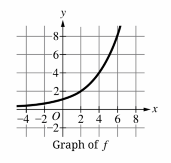
The correct option is (C).
Identify points from the graph: $(0, 1)$, $(2, 2)$, $(4, 4)$, and $(6, 8)$.
Calculate the ratio of consecutive outputs: $\frac{2}{1} = 2$, $\frac{4}{2} = 2$, and $\frac{8}{4} = 2$.
Since the input intervals are equal ($\Delta x = 2$), the output values are proportional.
A constant ratio over equal intervals is the defining property of an exponential function.
Option (B) describes quadratic behavior, which does not match the constant ratio observed.
Therefore, $f$ is exponential because its outputs grow by a common factor.

Question

A set of data is represented using a semi-log plot (not shown), in which the vertical axis is logarithmically scaled. The points on the semi-log plot appear to follow a decreasing linear pattern. Which of the following function types best models the set of data?

(A) Linear
(B) Exponential growth
(C) Exponential decay
(D) Logarithmic

▶️ Answer/Explanation

Detailed solution

The correct answer is (C) Exponential decay.
In a semi-log plot, the vertical axis represents $\log(y)$ and the horizontal axis represents $x$.
A linear pattern on this plot follows the equation $\log(y) = mx + b$.
Converting from logarithmic to exponential form gives $y = 10^{mx + b}$, which is an exponential function.
Since the pattern is decreasing, the slope $m$ must be negative ($m < 0$).
An exponential function with a negative growth rate represents exponential decay.
Therefore, the data is best modeled by an exponential decay function.

Question

The table gives the average rates of change for the functions $f$, $g$, $h$, and $k$ for certain intervals of $x$. Which of the functions is best modeled by a piecewise-linear function with two linear segments with different slopes?

(A) $f$
(B) $g$
(C) $h$
(D) $k$

▶️ Answer/Explanation

Detailed solution

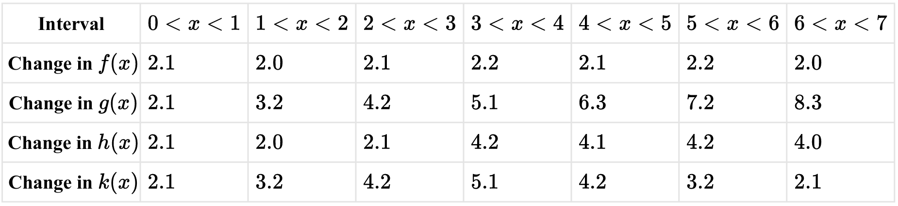
For a linear function, the rate of change remains constant.
A piecewise-linear function with two segments must show two distinct constant rates.
Function $f$ has a nearly constant rate of $\approx 2.1$, suggesting a single linear model.
Function $g$ shows a constantly increasing rate, suggesting a quadratic model.
Function $h$ stays at $\approx 2.1$ for $0 < x < 3$ and then jumps to $\approx 4.1$ for $3 < x < 7$.
This clear shift between two stable values identifies two linear segments with different slopes.
Function $k$ increases and then decreases, which is characteristic of a single nonlinear curve.
Therefore, $h$ is the best fit for a piecewise-linear model with two segments.

Question

Let $f$ be an increasing function defined for $x > 0$. The table gives values for $f(x)$ at selected values of $x$. The function $g$ is given by $g(x) = 0.25x^3 – 9.5x^2 + 110x – 399$.

Part A

(i) The function $h$ is defined by $h(x) = (g \circ f)(x) = g(f(x))$. Find the value of $h(8)$ as a decimal approximation, or indicate that it is not defined.

(ii) Find the value of $f^{-1}(20)$, or indicate that it is not defined.

Part B

(i) Find all values of $x$, as decimal approximations, for which $g(x) = -45$, or indicate there are no such values.

(ii) Determine the end behavior of $g$ as $x$ increases without bound. Express your answer using the mathematical notation of a limit.

Part C

(i) Use the table of values of $f(x)$ to determine if $f$ is best modeled by a linear, quadratic, exponential, or logarithmic function.

(ii) Give a reason for your answer based on the relationship between the change in the output values of $f$ and the change in the input values of $f$.

▶️ Answer/Explanation

Detailed solution

Part A

(i) From the table, we find $f(8) = 15$.

Substitute $15$ into the function $g(x)$: $h(8) = g(15) = 0.25(15)^3 – 9.5(15)^2 + 110(15) – 399$.

$h(8) = 0.25(3375) – 9.5(225) + 1650 – 399$.

$h(8) = 843.75 – 2137.5 + 1650 – 399$.

$h(8) = -42.75$.

(ii) To find $f^{-1}(20)$, we look for the $x$ value where $f(x) = 20$.

From the table, $f(16) = 20$.

Therefore, $f^{-1}(20) = 16$.

Part B

(i) We solve the equation $0.25x^3 – 9.5x^2 + 110x – 399 = -45$.

Set the equation to zero: $0.25x^3 – 9.5x^2 + 110x – 354 = 0$.

Using numerical methods or a graphing calculator, the real solutions are approximately:

$x \approx 5.242$

$x \approx 12.188$

$x \approx 20.570$

(ii) The end behavior of a polynomial is determined by its leading term, $0.25x^3$.

Since the leading coefficient is positive and the degree is odd, as $x \to \infty$, $g(x) \to \infty$.

The limit notation is $\lim_{x \to \infty} g(x) = \infty$.

Part C

(i) The function $f$ is best modeled by a logarithmic function.

(ii) In a logarithmic model, constant changes in the output values correspond to proportional changes in the input values.

As the output $f(x)$ increases by a constant $5$ ($0, 5, 10, 15 \dots$),

The input $x$ values are multiplied by a constant factor of $2$ ($1, 2, 4, 8 \dots$).

This constant ratio of inputs for constant additions of outputs is the hallmark of logarithmic growth.

Question

A graphing calculator is required for these questions.

Let $f$ be an increasing function defined for $x \ge 0$. The table gives values of $f(x)$ at selected values of $x$. The function $g$ is given by $g(x) = \frac{x^3 – 14x – 27}{x+2}$.

(A) (i) The function $h$ is defined by $h(x) = (g \circ f)(x) = g(f(x))$. Find the value of $h(5)$ as a decimal approximation, or indicate that it is not defined.

(ii) Find the value of $f^{-1}(4)$, or indicate that it is not defined.

(B) (i) Find all values of $x$, as decimal approximations, for which $g(x) = 3$, or indicate there are no such values.

(ii) Determine the end behavior of $g$ as $x$ decreases without bound. Express your answer using the mathematical notation of a limit.

(C) (i) Use the table of values of $f(x)$ to determine if $f$ is best modeled by a linear, quadratic, exponential, or logarithmic function.

(ii) Give a reason for your answer based on the relationship between the change in the output values of $f$ and the change in the input values of $f$.

▶️ Answer/Explanation

Detailed solution

(A) (i)
First, evaluate the inner function $f(5)$ using the table: $f(5) = 34$.
Next, substitute this value into $g(x)$ to find $h(5) = g(34)$.
$g(34) = \frac{34^3 – 14(34) – 27}{34 + 2}$
$g(34) = \frac{39304 – 476 – 27}{36} = \frac{38801}{36}$
$h(5) \approx 1077.806$

(A) (ii)
To find $f^{-1}(4)$, we look for the input value $x$ in the table that produces an output of $4$.
The table shows that $f(3) = 4$.
Therefore, $f^{-1}(4) = 3$.

(B) (i)
Set $g(x) = 3$ and solve for $x$:
$\frac{x^3 – 14x – 27}{x + 2} = 3$
Multiply both sides by $(x+2)$: $x^3 – 14x – 27 = 3(x + 2)$
Simplify: $x^3 – 14x – 27 = 3x + 6$
Rearrange into polynomial form: $x^3 – 17x – 33 = 0$
Using a graphing calculator to find the zero of this polynomial:
$x \approx 4.879$

(B) (ii)
We evaluate the limit as $x \to -\infty$ for $g(x)$.
$\lim_{x \to -\infty} \frac{x^3 – 14x – 27}{x + 2}$
By examining the leading terms, the function behaves like $\frac{x^3}{x} = x^2$ for large absolute values of $x$.
As $x \to -\infty$, $x^2 \to \infty$.
$\lim_{x \to -\infty} g(x) = \infty$

(C) (i)
Calculate the first differences of $f(x)$: $(-5) – (-10) = 5$, $4 – (-5) = 9$, $17 – 4 = 13$, $34 – 17 = 17$.
Calculate the second differences: $9 – 5 = 4$, $13 – 9 = 4$, $17 – 13 = 4$.
Since the second differences are constant, $f$ is best modeled by a quadratic function.

(C) (ii)
The model is quadratic because for equal intervals of the input values $x$ (step size of $1$), the rate of change of the output values increases by a constant amount (constant second difference of $4$).

AP Precalculus -1.13 Function Models: Selection and Assumptions- MCQ Exam Style Questions - Effective Fall 2023