AP Precalculus -1.14 Function Models: Construction and Application- FRQ Exam Style Questions - Effective Fall 2023

AP Precalculus -1.14 Function Models: Construction and Application- FRQ Exam Style Questions – Effective Fall 2023

AP Precalculus -1.14 Function Models: Construction and Application- FRQ Exam Style Questions – AP Precalculus- per latest AP Precalculus Syllabus.

AP Precalculus – FRQ Exam Style Questions- All Topics

Question

A restaurant added cheesecake to their menu. On the initial day $(t = 0)$ they sold 11 cheesecakes. 40 days later $(t = 40)$ they sold 62 cheesecakes. Twelve days after that $(t = 52)$ they sold 49 cheesecakes.

The number of cheesecakes sold can be modeled by the quadratic function $C(t) = at^2 + bt + c$ where $C(t)$ is the number of cheesecakes sold on day $t$.

(A)
(i) Use the given data to write three equations that can be used to find the values for constants $a, b,$ and $c$ in the expression for $C(t)$.
(ii) Find the values for $a, b,$ and $c$ as decimal approximations.

(B)
(i) Use the given data to find the average rate of change of the number of cheesecakes sold, in cheesecakes per day, from $t = 40$ to $t = 52$. Express your answer as a decimal approximation. Show the computations that lead to your answer.
(ii) Use the average rate of change found in (i) to estimate the number of cheesecakes sold on day $t = 45$. Show the work that leads to your answer.
(iii) Compare the estimate found in (ii) to the value given by the model $C(t)$. Using characteristics of the average rate of change and characteristics of the quadratic model, explain why the two estimates differ.

(C) Explain how the range values of the function should be limited by the context of the problem.

Most-appropriate topic codes (AP Precalculus CED):

• 1.14: Function Model Construction and Application – part A, B
• 1.3: Rates of Change in Linear and Quadratic Functions – part B
• 1.13: Function Model Selection and Assumption Articulation – part C

▶️ Answer/Explanation

A (i)
Given $C(0) = 11$, $C(40) = 62$, and $C(52) = 49$. The three equations are: \[ a(0)^2 + b(0) + c = 11 \] \[ a(40)^2 + b(40) + c = 62 \] \[ a(52)^2 + b(52) + c = 49 \]
✅ Answer: $c = 11$, $1600a + 40b + c = 62$, $2704a + 52b + c = 49$.

A (ii)
From the first equation, $c = 11$. Substituting $c=11$ into the other equations: $1600a + 40b = 51$ $2704a + 52b = 38$ Solving this system (using a calculator or elimination): Subtract equations: $-1104a + (-12b) = 13$ or solve directly. Using linear regression or system solving yields: $a = -0.04535… \approx -0.045$ $b = 3.08910… \approx 3.089$ $c = 11$
✅ Answer: $a \approx -0.045$, $b \approx 3.089$, $c = 11$.

B (i)
The average rate of change from $t=40$ to $t=52$ is: \[ \frac{C(52) – C(40)}{52 – 40} = \frac{49 – 62}{12} = -\frac{13}{12} \approx -1.083 \]
✅ Answer: $-1.083$ cheesecakes per day.

B (ii)
Using the estimated AROC to predict sales at $t=45$, which is 5 days after $t=40$: \[ C(45) \approx C(40) + (\text{AROC}) \times (45 – 40) \] \[ C(45) \approx 62 + (-1.083…)(5) = 62 – 5.41666… = 56.5833… \]
✅ Answer: Approximately 56 or 57 cheesecakes.

B (iii)
The actual model value: $C(45) = -0.045(45)^2 + 3.089(45) + 11 \approx 58.171$. The estimate from the AROC (56.583) is less than the model’s value (58.171). The quadratic model $C(t)$ opens downward ($a < 0$), so it is concave down. For a concave down function, the secant line connecting two points lies below the graph of the function on the interval. Since the estimate uses the linear secant line, it underestimates the true value of the function.
✅ Answer: The AROC estimate (≈56.6) is less than the model value (≈58.2). This is because the quadratic model is concave down, so the secant line is below the curve, producing an underestimate.

C
In the context, the restaurant cannot sell a negative number of cheesecakes. The range of $C(t)$ should be limited to non-negative values. The model yields a maximum value and eventually decreases, but only values of $C(t) \ge 0$ are meaningful.
✅ Answer: The range should be limited to $[0, \text{maximum}]$ or non-negative values, as you cannot sell a negative number of cheesecakes.

Question

The table gives the number of ice cream cones sold by a food vendor. On the initial day $t = 0$ when the vendor added ice cream cones to the menu, the vendor sold 14 ice cream cones. Thirty-five days later $t = 35$, the vendor sold 57 ice cream cones. Ten days after that $t = 45$, the vendor sold 46 ice cream cones.

The number of ice cream cones sold can be modeled by the quadratic function $I$ given by $I(t) = at^2 + bt + c$, where $I(t)$ is the number of ice cream cones sold on day $t$.

(A)

(i) Use the given data to write three equations that can be used to find the values for constants $a$, $b$, and $c$ in the expression for $I(t)$.

(ii) Find the values for $a$, $b$, and $c$ as decimal approximations.

(B)

(i) Use the given data to find the average rate of change of the number of ice cream cones sold, in cones per day, from $t = 35$ to $t = 45$ days. Express your answer as a decimal approximation. Show the computations that lead to your answer.

(ii) Use the average rate of change found in (i) to estimate the number of ice cream cones sold on day $t = 40$. Show the work that leads to your answer.

(iii) Compare the estimate found in (ii) to the value given by the model, $I(40)$. Using characteristics of the average rate of change and characteristics of the quadratic model, explain why the two estimates differ.

(C)

Explain how the range values of the function $I$ should be limited by the context of the problem.

Most-appropriate topic codes (AP Precalculus CED):

• 1.14: Function Model Construction and Application — parts (A), (B)(iii), (C)
• 2.2: Change in Linear and Exponential Functions — parts (B)(i), (B)(ii)
• 2.6: Competing Function Model Validation — part (B)(iii)

▶️ Answer/Explanation

(A)

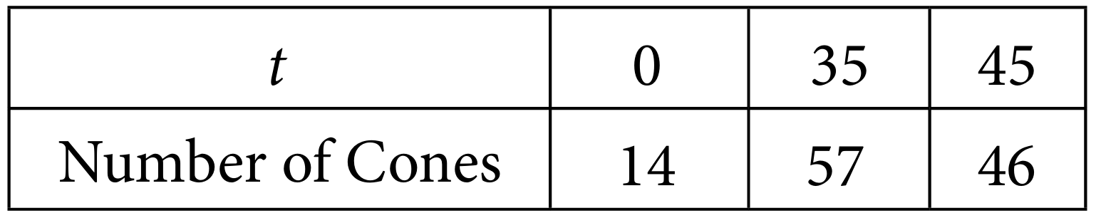
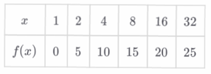
(i) Substituting the given data into the model $I(t) = at^2 + bt + c$:

When $t = 0$, $I(0) = 14$: $a(0)^2 + b(0) + c = 14 \Rightarrow c = 14$.
When $t = 35$, $I(35) = 57$: $a(35)^2 + b(35) + c = 57 \Rightarrow 1225a + 35b + c = 57$.
When $t = 45$, $I(45) = 46$: $a(45)^2 + b(45) + c = 46 \Rightarrow 2025a + 45b + c = 46$.

The three equations are:
$c = 14$
$1225a + 35b + 14 = 57$
$2025a + 45b + 14 = 46$
✅ Answer: The three equations are $c = 14$, $1225a + 35b = 43$, and $2025a + 45b = 32$.

(ii) Solve the system:

$1225a + 35b = 43$
$2025a + 45b = 32$

Multiply equation (1) by 9 and equation (2) by 7 to eliminate $b$: \[ 11025a + 315b = 387 \] \[ 14175a + 315b = 224 \] Subtract the first from the second: \[ 3150a = -163 \Rightarrow a = -\frac{163}{3150} \approx -0.051746\ldots \] Substitute $a$ into $1225a + 35b = 43$: \[ 1225(-0.051746) + 35b = 43 \Rightarrow -63.38885 + 35b = 43 \Rightarrow 35b = 106.38885 \Rightarrow b \approx 3.039681 \] Thus, \[ a \approx -0.052, \quad b \approx 3.040, \quad c = 14 \] ✅ Answer: $\boxed{a \approx -0.052,\ b \approx 3.040,\ c = 14}$ (or $a \approx -0.0517,\ b \approx 3.0397,\ c = 14$).

(B)

(i) Average rate of change from $t = 35$ to $t = 45$: \[ \frac{I(45) – I(35)}{45 – 35} = \frac{46 – 57}{10} = \frac{-11}{10} = -1.1 \] ✅ Answer: $\boxed{-1.1}$ cones per day.

(ii) Using the average rate of change: \[ I(40) \approx I(35) + (-1.1)(40 – 35) = 57 + (-1.1)(5) = 57 – 5.5 = 51.5 \] ✅ Answer: $\boxed{51.5}$ cones (approximately 51 or 52 cones).

(iii) Using the model: \[ I(40) \approx -0.052(40)^2 + 3.040(40) + 14 = -0.052(1600) + 121.6 + 14 = -83.2 + 135.6 = 52.4 \] More precisely with stored values: $I(40) \approx 52.794$.
The estimate from the average rate of change (51.5) is less than $I(40) \approx 52.8$.
Explanation: The average rate of change gives the slope of the secant line between $t = 35$ and $t = 45$. Since the quadratic model has $a < 0$, its graph is concave down. On the interval $(35, 45)$, the secant line lies below the graph. Therefore, the linear estimate using the average rate of change underestimates the actual value given by the concave-down quadratic at $t = 40$.
✅ Answer: The secant-line estimate is lower because the quadratic is concave down.

(C) The range of $I$ is limited by the context:

The number of cones sold cannot be negative: $I(t) \ge 0$.
Since $a < 0$, the quadratic has a maximum. From the model, the vertex gives the maximum number of cones sold. The vertex $t = -\frac{b}{2a} \approx 29.23$ yields $I_{\text{max}} \approx 58.64$.

Thus, a reasonable range is $0 \le I(t) \le 59$ (whole cones).
✅ Answer: The range is limited to non‑negative integers up to about 59 cones.

Question

Let $f$ be an increasing function defined for $x > 0$. The table gives values for $f(x)$ at selected values of $x$. The function $g$ is given by $g(x) = 0.25x^3 – 9.5x^2 + 110x – 399$.

Part A

(i) The function $h$ is defined by $h(x) = (g \circ f)(x) = g(f(x))$. Find the value of $h(8)$ as a decimal approximation, or indicate that it is not defined.

(ii) Find the value of $f^{-1}(20)$, or indicate that it is not defined.

Part B

(i) Find all values of $x$, as decimal approximations, for which $g(x) = -45$, or indicate there are no such values.

(ii) Determine the end behavior of $g$ as $x$ increases without bound. Express your answer using the mathematical notation of a limit.

Part C

(i) Use the table of values of $f(x)$ to determine if $f$ is best modeled by a linear, quadratic, exponential, or logarithmic function.

(ii) Give a reason for your answer based on the relationship between the change in the output values of $f$ and the change in the input values of $f$.

▶️ Answer/Explanation

Detailed solution

Part A

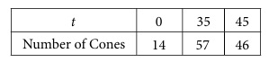
(i) From the table, we find $f(8) = 15$.

Substitute $15$ into the function $g(x)$: $h(8) = g(15) = 0.25(15)^3 – 9.5(15)^2 + 110(15) – 399$.

$h(8) = 0.25(3375) – 9.5(225) + 1650 – 399$.

$h(8) = 843.75 – 2137.5 + 1650 – 399$.

$h(8) = -42.75$.

(ii) To find $f^{-1}(20)$, we look for the $x$ value where $f(x) = 20$.

From the table, $f(16) = 20$.

Therefore, $f^{-1}(20) = 16$.

Part B

(i) We solve the equation $0.25x^3 – 9.5x^2 + 110x – 399 = -45$.

Set the equation to zero: $0.25x^3 – 9.5x^2 + 110x – 354 = 0$.

Using numerical methods or a graphing calculator, the real solutions are approximately:

$x \approx 5.242$

$x \approx 12.188$

$x \approx 20.570$

(ii) The end behavior of a polynomial is determined by its leading term, $0.25x^3$.

Since the leading coefficient is positive and the degree is odd, as $x \to \infty$, $g(x) \to \infty$.

The limit notation is $\lim_{x \to \infty} g(x) = \infty$.

Part C

(i) The function $f$ is best modeled by a logarithmic function.

(ii) In a logarithmic model, constant changes in the output values correspond to proportional changes in the input values.

As the output $f(x)$ increases by a constant $5$ ($0, 5, 10, 15 \dots$),

The input $x$ values are multiplied by a constant factor of $2$ ($1, 2, 4, 8 \dots$).

This constant ratio of inputs for constant additions of outputs is the hallmark of logarithmic growth.

Question

A graphing calculator is required for these questions.

Let $f$ be an increasing function defined for $x \ge 0$. The table gives values of $f(x)$ at selected values of $x$. The function $g$ is given by $g(x) = \frac{x^3 – 14x – 27}{x+2}$.

(A) (i) The function $h$ is defined by $h(x) = (g \circ f)(x) = g(f(x))$. Find the value of $h(5)$ as a decimal approximation, or indicate that it is not defined.

(ii) Find the value of $f^{-1}(4)$, or indicate that it is not defined.

(B) (i) Find all values of $x$, as decimal approximations, for which $g(x) = 3$, or indicate there are no such values.

(ii) Determine the end behavior of $g$ as $x$ decreases without bound. Express your answer using the mathematical notation of a limit.

(C) (i) Use the table of values of $f(x)$ to determine if $f$ is best modeled by a linear, quadratic, exponential, or logarithmic function.

(ii) Give a reason for your answer based on the relationship between the change in the output values of $f$ and the change in the input values of $f$.

▶️ Answer/Explanation

Detailed solution

(A) (i)
First, evaluate the inner function $f(5)$ using the table: $f(5) = 34$.
Next, substitute this value into $g(x)$ to find $h(5) = g(34)$.
$g(34) = \frac{34^3 – 14(34) – 27}{34 + 2}$
$g(34) = \frac{39304 – 476 – 27}{36} = \frac{38801}{36}$
$h(5) \approx 1077.806$

(A) (ii)
To find $f^{-1}(4)$, we look for the input value $x$ in the table that produces an output of $4$.
The table shows that $f(3) = 4$.
Therefore, $f^{-1}(4) = 3$.

(B) (i)
Set $g(x) = 3$ and solve for $x$:
$\frac{x^3 – 14x – 27}{x + 2} = 3$
Multiply both sides by $(x+2)$: $x^3 – 14x – 27 = 3(x + 2)$
Simplify: $x^3 – 14x – 27 = 3x + 6$
Rearrange into polynomial form: $x^3 – 17x – 33 = 0$
Using a graphing calculator to find the zero of this polynomial:
$x \approx 4.879$

(B) (ii)
We evaluate the limit as $x \to -\infty$ for $g(x)$.
$\lim_{x \to -\infty} \frac{x^3 – 14x – 27}{x + 2}$
By examining the leading terms, the function behaves like $\frac{x^3}{x} = x^2$ for large absolute values of $x$.
As $x \to -\infty$, $x^2 \to \infty$.
$\lim_{x \to -\infty} g(x) = \infty$

(C) (i)
Calculate the first differences of $f(x)$: $(-5) – (-10) = 5$, $4 – (-5) = 9$, $17 – 4 = 13$, $34 – 17 = 17$.
Calculate the second differences: $9 – 5 = 4$, $13 – 9 = 4$, $17 – 13 = 4$.
Since the second differences are constant, $f$ is best modeled by a quadratic function.

(C) (ii)
The model is quadratic because for equal intervals of the input values $x$ (step size of $1$), the rate of change of the output values increases by a constant amount (constant second difference of $4$).

AP Precalculus -1.14 Function Models: Construction and Application- FRQ Exam Style Questions - Effective Fall 2023