Constructing Models Using Transformations of Parent Functions
A mathematical model of a data set or a contextual scenario can be constructed by applying transformations to a parent function.
Parent functions, such as linear, quadratic, square root, and rational functions, provide basic shapes that can be adjusted to fit real data.
By using translations, dilations, and reflections, the parent function can be shifted and scaled so that it better represents the situation.
A general transformed model can be written as
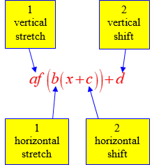
\( \mathrm{ \displaystyle g(x) = a\,f(bx + h) + k } \)
Each parameter allows the model to match features such as starting values, maximum or minimum values, growth or decay rates, and physical constraints.
Example
A projectile is launched from a platform 10 meters above the ground.
The parent function for vertical motion is \( \mathrm{f(x) = -x^2} \).
Construct a model for the height of the projectile.
▶️ Answer/Explanation
The negative sign models downward opening motion.
The starting height of 10 meters is represented by a vertical translation.
\( \mathrm{ \displaystyle h(x) = -x^2 + 10 } \)
Conclusion
The model is constructed by transforming the parent quadratic function upward by 10 units.
Example
The cost of renting a bike increases steadily, starting with a fixed initial fee.
The parent function is \( \mathrm{f(x) = x} \).
Construct a model for the total cost.
▶️ Answer/Explanation
The constant rate of increase is represented by a vertical dilation.
The fixed starting fee is represented by a vertical translation.
\( \mathrm{ \displaystyle C(x) = 5x + 20 } \)
Conclusion
The model is formed by transforming the parent linear function to match the context.
Constructing Models Using Technology and Regression
A model of a data set can be constructed using technology and regression techniques.
Regression finds a function that best fits a set of data points by minimizing the overall error between the model and the data.
Different types of regression models are chosen based on the shape and behavior of the data.
Common Regression Models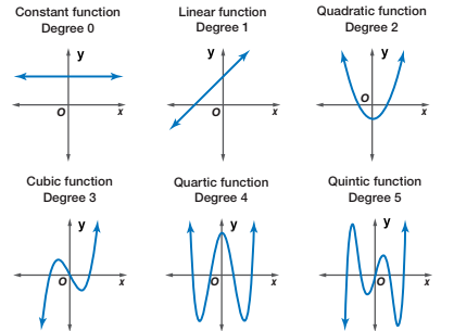
• Linear regression: used when the data shows an approximately constant rate of change
• Quadratic regression: used when the data has a single maximum or minimum and is roughly symmetric
• Cubic regression: used when the data changes direction more than once
• Quartic regression: used when the data shows multiple turning points
Technology such as graphing calculators or software is used to determine the regression equation.
The chosen model should make sense mathematically and within the context of the data.
Example
A data set shows the distance traveled by a car over time.
The data points lie close to a straight line.
▶️ Answer/Explanation
Because the rate of change is approximately constant, a linear regression model is appropriate.
Using technology, a possible model is
\( \mathrm{ \displaystyle d(t) = 55t + 10 } \)
This equation estimates the distance for any given time value.
Example
A data set models the height of a ball over time.
The data rises to a maximum value and then decreases.
▶️ Answer/Explanation
The shape suggests a quadratic relationship.
Using quadratic regression, a possible model is
\( \mathrm{ \displaystyle h(t) = -4.9t^2 + 18t + 2 } \)
The maximum value represents the greatest height reached.
Constructing Models Using Piecewise-Defined Functions
A piecewise-defined function is a function that is defined by different rules on different intervals of its domain.
A piecewise model is used when a single function rule cannot accurately describe the entire data set or contextual scenario.
Such models are constructed by combining multiple modeling techniques, such as linear, quadratic, or constant functions, each applied where it best fits the situation.
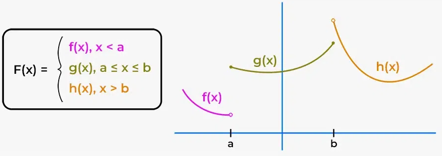
A general piecewise-defined function is written as
\( \mathrm{ \displaystyle f(x)= \begin{cases} \text{rule}_1, & \text{for } x \text{ in interval}_1 \\ \text{rule}_2, & \text{for } x \text{ in interval}_2 \\ \vdots \end{cases} } \)
Each rule reflects the behavior of the model over a specific interval, based on context, data trends, or physical constraints.
Piecewise models are common in scenarios involving pricing plans, motion with changing speeds, or processes with distinct phases.
Example
A parking garage charges a flat fee for the first hour and then charges by the hour afterward.
The cost is ₹50 for up to 1 hour, and ₹30 per hour for each additional hour.
▶️ Answer/Explanation
Let \( \mathrm{x} \) represent time in hours.
The model is
\( \mathrm{ \displaystyle C(x)= \begin{cases} 50, & 0 < x \le 1 \\ 50 + 30(x-1), & x > 1 \end{cases} } \)
Conclusion
Different linear rules are used to model the cost before and after one hour.
Example
A car accelerates uniformly for the first 5 seconds and then moves at a constant speed.
The distance traveled is modeled using different rules for each phase.
▶️ Answer/Explanation
Let \( \mathrm{t} \) represent time in seconds.
A suitable model is
\( \mathrm{ \displaystyle s(t)= \begin{cases} 2t^2, & 0 \le t \le 5 \\ 50 + 20(t-5), & t > 5 \end{cases} } \)
Conclusion
The quadratic rule models acceleration, while the linear rule models constant speed.
Constructing a Rational Function Model from a Context
In many real-world situations, two quantities vary in such a way that one quantity is proportional to the reciprocal of another quantity, or to the reciprocal of a power of another quantity.
Such relationships are commonly modeled using rational functions.
A rational function is especially useful when quantities are inversely proportional.
Inverse Proportionality
If a quantity \( \mathrm{y} \) is inversely proportional to a quantity \( \mathrm{x} \), then the relationship can be written as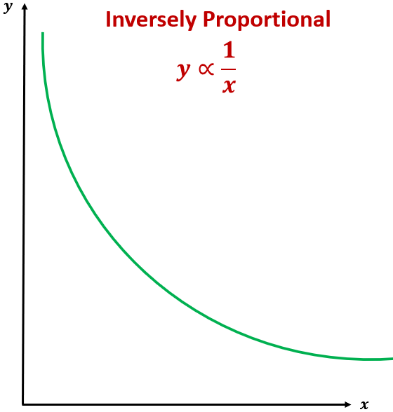
\( \mathrm{ \displaystyle y = \dfrac{k}{x} } \)
where \( \mathrm{k} \) is a constant of proportionality.
If the inverse relationship involves a square, the model becomes
\( \mathrm{ \displaystyle y = \dfrac{k}{x^2} } \)
This type of model appears in physical laws such as gravitational force and electromagnetic force, where force decreases rapidly as distance increases.
Constructing a rational function model involves:
• Identifying the inverse relationship
• Writing a general rational expression
• Using given data to determine the constant of proportionality
Example :
The intensity \( \mathrm{I} \) of a signal is inversely proportional to the distance \( \mathrm{d} \) from the source.
When the distance is 4 units, the intensity is 20 units.
Construct a rational function model.
▶️ Answer/Explanation
Since the relationship is inversely proportional, start with
\( \mathrm{ \displaystyle I = \dfrac{k}{d} } \)
Substitute the given values:
\( \mathrm{ \displaystyle 20 = \dfrac{k}{4} } \)
Solve for \( \mathrm{k} \):
\( \mathrm{ \displaystyle k = 80 } \)
Model
\( \mathrm{ \displaystyle I(d) = \dfrac{80}{d} } \)
Example :
The force \( \mathrm{F} \) between two objects is inversely proportional to the square of the distance \( \mathrm{r} \) between them.
When the distance is 2 meters, the force is 50 newtons.
Construct a rational function model.
▶️ Answer/Explanation
Since force is inversely proportional to the square of distance, start with
\( \mathrm{ \displaystyle F = \dfrac{k}{r^2} } \)
Substitute the given values:
\( \mathrm{ \displaystyle 50 = \dfrac{k}{2^2} } \)
Solve for \( \mathrm{k} \):
\( \mathrm{ \displaystyle k = 200 } \)
Model
\( \mathrm{ \displaystyle F(r) = \dfrac{200}{r^2} } \)
The model shows that as distance increases, the force decreases rapidly.
Applying a Function Model to a Context or Data Set
Once a function model has been constructed from a data set or contextual scenario, it can be used to analyze behavior, answer questions, and make predictions.
A function model represents how two quantities vary together, allowing us to interpret numerical results in meaningful, real-world terms.
Using a Model to Draw Conclusions
A function model can be used to:
• Predict output values for given input values
• Estimate values outside the observed data range (with caution)
• Determine rates of change and average rates of change
• Describe how the rate of change itself is changing
When interpreting results, it is essential to include appropriate units, which should be extracted or inferred from the context.
The meaning of a numerical answer depends on what the variables represent.
Example :
A company models its daily profit (in dollars) using the function
\( \mathrm{ \displaystyle P(x) = 120x – 500 } \)
where \( \mathrm{x} \) is the number of units sold.
Use the model to find the profit when 15 units are sold.
▶️ Answer/Explanation
Substitute \( \mathrm{x = 15} \) into the model:
\( \mathrm{ \displaystyle P(15) = 120(15) – 500 } \)
\( \mathrm{ \displaystyle P(15) = 1800 – 500 = 1300 } \)
Conclusion
When 15 units are sold, the model predicts a profit of $1300.
Example :
The height of a ball (in meters) after \( \mathrm{t} \) seconds is modeled by
\( \mathrm{ \displaystyle h(t) = -5t^2 + 20t + 1 } \)
Find and interpret the average rate of change of the height between \( \mathrm{t = 1} \) and \( \mathrm{t = 3} \).
▶️ Answer/Explanation
Compute the function values:
\( \mathrm{ \displaystyle h(1) = -5(1)^2 + 20(1) + 1 = 16 } \)
\( \mathrm{ \displaystyle h(3) = -5(3)^2 + 20(3) + 1 = 16 } \)
Compute the average rate of change:
\( \mathrm{ \displaystyle \dfrac{h(3) – h(1)}{3 – 1} = \dfrac{16 – 16}{2} = 0 } \)
Conclusion
The average rate of change is 0 meters per second, meaning the ball is at the same height at \( \mathrm{t = 1} \) and \( \mathrm{t = 3} \).
This reflects the changing rate of change typical of quadratic motion.