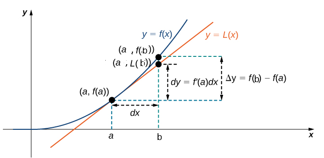
Average Rate of Change
The average rate of change of a function over an interval of its domain is the constant rate of change that produces the same total change in output as the function does over that interval.
It is calculated as the ratio of the change in output values to the change in input values over the interval.

\( \text{Average rate of change} = \dfrac{f(b) – f(a)}{b – a} \)
Geometrically, this value represents the slope of the secant line connecting the points \( (a, f(a)) \) and \( (b, f(b)) \) on the graph of the function.
In real world contexts, the average rate of change can represent quantities such as average speed, average growth, or average cost over a given interval.
Example:
Find the average rate of change of the function \( f(x) = x^2 + 3x \) over the interval \( [1, 4] \).
▶️ Answer/Explanation
Compute \( f(4) \)
\( f(4) = 4^2 + 3(4) = 16 + 12 = 28 \)
Compute \( f(1) \)
\( f(1) = 1^2 + 3(1) = 1 + 3 = 4 \)
Compute average rate of change
\( \dfrac{28 – 4}{4 – 1} = \dfrac{24}{3} = 8 \)
Final answer:
The average rate of change over the interval is \( 8 \).
Example:
The position of a cyclist is given by \( s(t) = 5t^2 \), where \( s \) is in meters and \( t \) is in seconds. Find the average velocity between \( t = 2 \) and \( t = 6 \).
▶️ Answer/Explanation
Compute \( s(6) \)
\( s(6) = 5(6)^2 = 5(36) = 180 \)
Compute \( s(2) \)
\( s(2) = 5(2)^2 = 5(4) = 20 \)
Compute average velocity
\( \dfrac{180 – 20}{6 – 2} = \dfrac{160}{4} = 40 \)
Final answer:
The average velocity between \( t = 2 \) and \( t = 6 \) is \( 40 \ \text{m/s} \).
Rate of Change at a Point
The rate of change of a function at a point measures how fast the output value of the function changes with respect to the input value at that specific point.
If the function is written as \( y = f(x) \), then the rate of change at the input value \( x = a \) describes how \( f(x) \) would change for very small changes in \( x \) near \( a \).
Mathematically, the rate of change at a point can be approximated using average rates of change over small intervals containing that point.
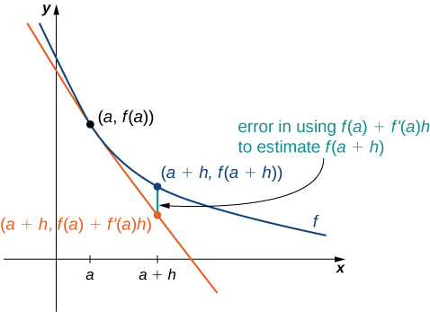
\( \text{Average rate of change on } [a, a+h] = \dfrac{f(a+h) – f(a)}{h} \)
As the interval length \( h \) becomes smaller, this average rate of change provides a better approximation of the rate of change at \( x = a \).
Graphically, the rate of change at a point corresponds to the slope of the tangent line to the graph at that point.
The rates of change at two different points can be compared by computing average rates of change over sufficiently small intervals around each point.
Example:
Approximate the rate of change of the function \( f(x) = x^2 \) at \( x = 3 \) using the interval \( [3, 3.01] \).
▶️ Answer/Explanation
Compute function values
\( f(3) = 3^2 = 9 \)
\( f(3.01) = (3.01)^2 = 9.0601 \)
Compute average rate of change
\( \dfrac{9.0601 – 9}{3.01 – 3} = \dfrac{0.0601}{0.01} = 6.01 \)
Interpretation
The rate of change of \( f(x) = x^2 \) at \( x = 3 \) is approximately \( 6.01 \).
Example:
Compare the rates of change of the function \( g(x) = x^3 \) at \( x = 1 \) and \( x = 2 \) using small intervals of length \( 0.01 \).
▶️ Answer/Explanation
At \( x = 1 \)
\( g(1) = 1 \)
\( g(1.01) = (1.01)^3 = 1.030301 \)
Average rate of change:
\( \dfrac{1.030301 – 1}{0.01} = 3.0301 \)
At \( x = 2 \)
\( g(2) = 8 \)
\( g(2.01) = (2.01)^3 = 8.120601 \)
Average rate of change:
\( \dfrac{8.120601 – 8}{0.01} = 12.0601 \)
Conclusion
The rate of change at \( x = 2 \) is much larger than at \( x = 1 \), showing that the function changes more rapidly at larger input values.
Interpreting Rates of Change
Rates of change describe how two quantities vary together and measure how a change in one quantity affects another.
If a relationship is written as \( y = f(x) \), then the rate of change compares changes in the output \( y \) to changes in the input \( x \).
\( \text{Rate of change} = \dfrac{\Delta y}{\Delta x} = \dfrac{f(b) – f(a)}{b – a} \)
Positive Rate of Change
A rate of change is positive when an increase or decrease in one quantity causes the other quantity to increase or decrease in the same direction.
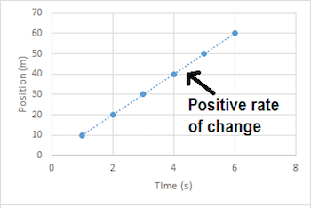
Graphically, a positive rate of change corresponds to a graph that rises from left to right.
Negative Rate of Change
A rate of change is negative when an increase in one quantity causes the other quantity to decrease.
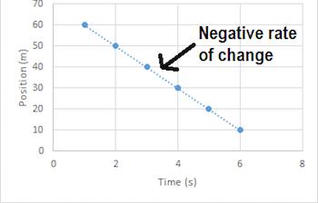
Graphically, a negative rate of change corresponds to a graph that falls from left to right.
Example:
The function \( f(x) = 5x \) models the distance traveled over time. Interpret the rate of change.
▶️ Answer/Explanation
The rate of change is the coefficient of \( x \), which is 5.
This means that for every increase of 1 unit in time, the distance increases by 5 units.
Since both quantities increase together, the rate of change is positive.
Example:
The temperature of a hot drink decreases over time and is modeled by \( T(t) = 80 – 3t \). Interpret the rate of change.
▶️ Answer/Explanation
The rate of change is \( -3 \).
This means that for every increase of 1 unit in time, the temperature decreases by 3 units.
Because one quantity increases while the other decreases, the rate of change is negative.