AP Precalculus -1.3 Rates of Change in Linear and Quadratic Functions- FRQ Exam Style Questions - Effective Fall 2023

AP Precalculus -1.3 Rates of Change in Linear and Quadratic Functions- FRQ Exam Style Questions – Effective Fall 2023

AP Precalculus -1.3 Rates of Change in Linear and Quadratic Functions- FRQ Exam Style Questions – AP Precalculus- per latest AP Precalculus Syllabus.

AP Precalculus – FRQ Exam Style Questions- All Topics

Question

The blades of an electric fan rotate in a clockwise direction and complete $5$ rotations every second. Point $B$ is on the tip of one of the fan blades and is located directly above the center of the fan at time $t = 0$ seconds. Point $B$ is $6$ inches from the center of the fan. The center of the fan is $20$ inches above a level table. The sinusoidal function $h$ models the distance between $B$ and the surface of the table in inches as a function of time $t$ in seconds.

(A) The graph of ℎ and its dashed midline for two full cycles is shown. Five points, 𝐹, 𝐺, 𝐽, 𝐾, and 𝑃 are labeled on the graph. No scale is indicated, and no axes are presented.
Determine the possible coordinates $(t, h(t))$ for the $5$ points: $F, G, J, K,$ and $P$.

(B) The function $h$ can be written in the form $h(t) = a \sin(b(t + c)) + d$. Find values of constants $a, b, c,$ and $d$.

(i) On the interval $(t_1, t_2)$, which of the following is true about $h$?
(A) $h$ is positive and increasing
(B) $h$ is positive and decreasing
(C) $h$ is negative and increasing
(D) $h$ is negative and decreasing

(ii) Describe how the rate of change of $h$ is changing on the interval $(t_1, t_2)$.

Most-appropriate topic codes (AP Precalculus CED):

• 3.7: Sinusoidal Function Context and Data Modeling – part A, part B
• 1.1: Change in Tandem – part C(i)
• 1.3: Rates of Change in Linear and Quadratic Functions – part C(ii)

▶️ Answer/Explanation

Detailed solution

(A)

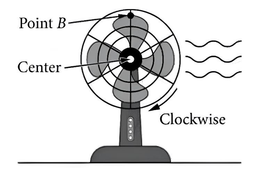
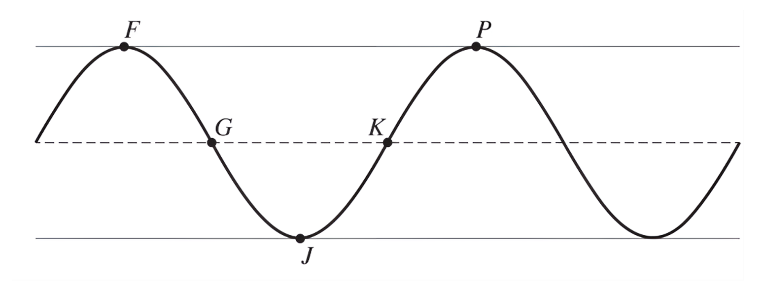
The center of the fan is $d = 20$ inches above the table. The radius of the fan blade is $r = 6$ inches, which is the amplitude $a$. The maximum height is $20 + 6 = 26$ inches and the minimum height is $20 – 6 = 14$ inches. The fan completes $5$ rotations per second, so the period is $T = \frac{1}{5} = 0.2$ seconds. Point $B$ starts at the maximum height at $t = 0$, so point $F$ is $(0, 26)$. Point $G$ is at the midline after $\frac{1}{4}$ of a period: $(\frac{0.2}{4}, 20) = (0.05, 20)$. Point $J$ is at the minimum after $\frac{1}{2}$ of a period: $(\frac{0.2}{2}, 14) = (0.1, 14)$. Point $K$ is at the midline after $\frac{3}{4}$ of a period: $(\frac{3 \times 0.2}{4}, 20) = (0.15, 20)$. Point $P$ is at the maximum after $1$ full period: $(0.2, 26)$. The coordinates are: $F(0, 26)$, $G(0.05, 20)$, $J(0.1, 14)$, $K(0.15, 20)$, and $P(0.2, 26)$.

(B)

The amplitude is $a = 6$. The vertical shift (midline) is $d = 20$. The period is $T = 0.2$, so the frequency constant is $b = \frac{2\pi}{0.2} = 10\pi$. Since the function starts at a maximum at $t=0$, it follows $h(t) = 6 \cos(10\pi t) + 20$. To write this as a sine function $h(t) = 6 \sin(10\pi(t + c)) + 20$, we use the identity $\cos(\theta) = \sin(\theta + \frac{\pi}{2})$. Setting $10\pi(t + c) = 10\pi t + \frac{\pi}{2}$, we find $10\pi c = \frac{\pi}{2}$, which gives $c = \frac{1}{20} = 0.05$. Thus, $a = 6$, $b = 10\pi$, $c = 0.05$, and $d = 20$.

(C)

(i) On the interval $(t_1, t_2)$, which is $(0.15, 0.2)$, the graph moves from the midline (point $K$) up to the maximum (point $P$). Throughout this interval, $h(t)$ is between $20$ and $26$, so it is positive. The function is moving upwards, so it is increasing. The correct option is (A) $h$ is positive and increasing.
(ii) On the interval $(t_1, t_2)$, the graph is concave down as it levels off toward the maximum. The slope (rate of change) is positive because the function is increasing. However, the slope is becoming less steep as it approaches the horizontal tangent at point $P$. Therefore, the rate of change of $h$ is decreasing on the interval $(t_1, t_2)$.

Question

An ecologist began studying a certain type of plant species in a wetlands area in 2013. In 2015 ($t=2$), there were 59 plants. In 2021 ($t=8$), there were 118 plants.

The number of plants in this species can be modeled by the function $P$ given by $P(t)=ab^t$, where $P(t)$ is the number of plants during year $t$, and $t$ is the number of years since 2013.

(A)
(i) Use the given data to write two equations that can be used to find the values for constants $a$ and $b$ in the expression for $P(t)$.
(ii) Find the values for $a$ and $b$ as decimal approximations.

(B)
(i) Use the given data to find the average rate of change of the number of plants, in plants per year, from $t=2$ to $t=8$ years. Express your answer as a decimal approximation. Show the computations that lead to your answer.
(ii) Use the average rate of change found in (i) to estimate the number of plants for $t=10$ years. Show the work that leads to your answer.
(iii) The average rate of change found in (i) can be used to estimate the number of plants during year $t$ for $t>10$ years. Will these estimates, found using the average rate of change, be less than or greater than the number of plants predicted by the model $P$ during year $t$ for $t>10$ years? Explain your reasoning.

(C)
For which $t$-value, $t=6$ years or $t=20$ years, should the ecologist have more confidence in when using the model $P$? Give a reason for your answer in the context of the problem.

Most-appropriate topic codes (AP Precalculus CED):

• 2.5: Exponential Function Context and Data Modeling – part A
• 1.2: Rates of Change – part B
• 1.3: Rates of Change in Linear and Quadratic Functions – part B(ii), B(iii)
• 1.13: Function Model Selection and Assumption Articulation – part C

▶️ Answer/Explanation

A (i)
Because $P(2)=59$ and $P(8)=118$, the two equations to find $a$ and $b$ are $ab^2=59$ and $ab^8=118$.
✅ Answer: $\boxed{ab^2=59 \text{ and } ab^8=118}$

A (ii)
Divide the second equation by the first: $\frac{ab^8}{ab^2} = \frac{118}{59} \implies b^6 = 2$.
$b = (2)^{1/6} \approx 1.122462$.
Substitute $b$ back into the first equation: $a = \frac{59}{b^2} \approx 46.828331$.
✅ Answer: $\boxed{a \approx 46.828, \; b \approx 1.122}$

B (i)
Average Rate of Change = $\frac{P(8)-P(2)}{8-2}$.
Calculation: $\frac{118-59}{6} = \frac{59}{6} \approx 9.833$.
✅ Answer: The average rate of change is $\boxed{9.833 \text{ plants per year}}$.

B (ii)
We can model this estimation using the point-slope form of the secant line: $y = P(2) + r(x-2)$, where $r \approx 9.833$.
For $t=10$: $y = 59 + 9.833(10-2) = 137.667$.
✅ Answer: The number of plants for $t=10$ years was approximately $\boxed{137 \text{ or } 138}$.

B (iii)
The estimate is less than the predicted model value.
Reasoning: The estimate using the average rate of change corresponds to the $y$-coordinate of a point on the secant line that passes through $(2, P(2))$ and $(8, P(8))$. Because an exponential growth graph like $P$ is concave up on the interval $(-\infty, \infty)$, the secant line lies below the curve outside of the interval $(2,8)$. Thus, for $t>10$, the secant line estimate represents an underprediction.

C
The ecologist should have more confidence in using the model for $t=6$ years.
Reasoning: It is appropriate to use the regression model to interpolate values at times that fall between the minimum time ($t=2$) and the maximum time ($t=8$) provided in the data. However, there is insufficient information to know how many years the exponential model can be reliably extended beyond $t=8$ to make reasonable predictions (extrapolation involves more risk and uncertainty).

Question

A restaurant added cheesecake to their menu. On the initial day $(t = 0)$ they sold 11 cheesecakes. 40 days later $(t = 40)$ they sold 62 cheesecakes. Twelve days after that $(t = 52)$ they sold 49 cheesecakes.

The number of cheesecakes sold can be modeled by the quadratic function $C(t) = at^2 + bt + c$ where $C(t)$ is the number of cheesecakes sold on day $t$.

(A)
(i) Use the given data to write three equations that can be used to find the values for constants $a, b,$ and $c$ in the expression for $C(t)$.
(ii) Find the values for $a, b,$ and $c$ as decimal approximations.

(B)
(i) Use the given data to find the average rate of change of the number of cheesecakes sold, in cheesecakes per day, from $t = 40$ to $t = 52$. Express your answer as a decimal approximation. Show the computations that lead to your answer.
(ii) Use the average rate of change found in (i) to estimate the number of cheesecakes sold on day $t = 45$. Show the work that leads to your answer.
(iii) Compare the estimate found in (ii) to the value given by the model $C(t)$. Using characteristics of the average rate of change and characteristics of the quadratic model, explain why the two estimates differ.

(C) Explain how the range values of the function should be limited by the context of the problem.

Most-appropriate topic codes (AP Precalculus CED):

• 1.14: Function Model Construction and Application – part A, B
• 1.3: Rates of Change in Linear and Quadratic Functions – part B
• 1.13: Function Model Selection and Assumption Articulation – part C

▶️ Answer/Explanation

A (i)
Given $C(0) = 11$, $C(40) = 62$, and $C(52) = 49$. The three equations are: \[ a(0)^2 + b(0) + c = 11 \] \[ a(40)^2 + b(40) + c = 62 \] \[ a(52)^2 + b(52) + c = 49 \]
✅ Answer: $c = 11$, $1600a + 40b + c = 62$, $2704a + 52b + c = 49$.

A (ii)
From the first equation, $c = 11$. Substituting $c=11$ into the other equations: $1600a + 40b = 51$ $2704a + 52b = 38$ Solving this system (using a calculator or elimination): Subtract equations: $-1104a + (-12b) = 13$ or solve directly. Using linear regression or system solving yields: $a = -0.04535… \approx -0.045$ $b = 3.08910… \approx 3.089$ $c = 11$
✅ Answer: $a \approx -0.045$, $b \approx 3.089$, $c = 11$.

B (i)
The average rate of change from $t=40$ to $t=52$ is: \[ \frac{C(52) – C(40)}{52 – 40} = \frac{49 – 62}{12} = -\frac{13}{12} \approx -1.083 \]
✅ Answer: $-1.083$ cheesecakes per day.

B (ii)
Using the estimated AROC to predict sales at $t=45$, which is 5 days after $t=40$: \[ C(45) \approx C(40) + (\text{AROC}) \times (45 – 40) \] \[ C(45) \approx 62 + (-1.083…)(5) = 62 – 5.41666… = 56.5833… \]
✅ Answer: Approximately 56 or 57 cheesecakes.

B (iii)
The actual model value: $C(45) = -0.045(45)^2 + 3.089(45) + 11 \approx 58.171$. The estimate from the AROC (56.583) is less than the model’s value (58.171). The quadratic model $C(t)$ opens downward ($a < 0$), so it is concave down. For a concave down function, the secant line connecting two points lies below the graph of the function on the interval. Since the estimate uses the linear secant line, it underestimates the true value of the function.
✅ Answer: The AROC estimate (≈56.6) is less than the model value (≈58.2). This is because the quadratic model is concave down, so the secant line is below the curve, producing an underestimate.

C
In the context, the restaurant cannot sell a negative number of cheesecakes. The range of $C(t)$ should be limited to non-negative values. The model yields a maximum value and eventually decreases, but only values of $C(t) \ge 0$ are meaningful.
✅ Answer: The range should be limited to $[0, \text{maximum}]$ or non-negative values, as you cannot sell a negative number of cheesecakes.

Question

A scientist is growing bacteria in a lab. After 2 hours there were 32 bacteria. After 6 hours there were 115 bacteria.

The number of bacteria can be modeled by the function $P(t) = ab^t$ , where $P(t)$ is the number of bacteria $t$ hours after he began.

(A)
(i) Use the given data to write two equations that can be used to find the values for constants $a$ and $b$ in the expression for $P(t)$.
(ii) Find the values for $a$ and $b$ as decimal approximations.

(B)
(i) Use the given data to find the average rate of change of the number of bacteria, in bacteria per hour, from $t = 2$ to $t = 6$ hours. Express your answer as a decimal approximation. Show the computations that lead to your answer.
(ii) Use the average rate of change in (i) to estimate the number of bacteria for $t = 9$ hours. Show the computations that lead to your answer.
(iii) The average rate of change found in (i) can be used to estimate the number of bacteria during hour $t$ for $t > 9$ hours. Will these estimates, found using the average rate of change, be less than or greater than the number of bacteria predicted by the model during the hour $t$ for $t > 9$ hours? Explain your reasoning.

(C) For which $t$-value, $t = 4$ hours or $t = 15$ hours, should the scientist have more confidence in when using the model $P$ ? Give a reason for your answer in the context of the problem.

Most-appropriate topic codes (AP Precalculus CED):

▶️ Answer/Explanation

A (i)
Using the model $P(t) = ab^t$: From the data, $P(2) = 32$ and $P(6) = 115$.
The two equations are: \[ ab^2 = 32 \] \[ ab^6 = 115 \]
✅ Answer: The system of equations is $ab^2 = 32$ and $ab^6 = 115$.

A (ii)
Divide the second equation by the first: \[ \frac{ab^6}{ab^2} = \frac{115}{32} \implies b^4 = \frac{115}{32} \] Taking the positive fourth root (since $b > 0$): \[ b = \left(\frac{115}{32}\right)^{1/4} \approx 1.377 \] Substitute $b$ into the first equation: \[ a(1.377)^2 = 32 \implies a \approx \frac{32}{1.896} \approx 16.880 \]
✅ Answer: $a \approx 16.880$, $b \approx 1.377$.

B (i)
The average rate of change (AROC) of $P$ from $t=2$ to $t=6$ is: \[ \frac{P(6) – P(2)}{6 – 2} = \frac{115 – 32}{4} = \frac{83}{4} = 20.75 \]
✅ Answer: The average rate of change is $20.75$ bacteria per hour.

B (ii)
Using the AROC, the change in bacteria from $t=2$ to $t=9$ is approximated by $20.75 \times (9-2) = 20.75 \times 7 = 145.25$. Estimated number of bacteria at $t=9$: \[ P(9) \approx P(2) + 145.25 = 32 + 145.25 = 177.25 \] Since bacteria count is discrete, this is approximately 177 or 178 bacteria.
✅ Answer: Approximately 177 bacteria.

B (iii)
The model $P(t)=ab^t$ is an exponential growth function. Exponential functions are concave up. The secant line used for the AROC estimate lies below the graph of a concave up function. Therefore, linear estimates based on the secant line will be less than the actual values predicted by the model.
✅ Answer: The estimates using the average rate of change will be less than the number of bacteria predicted by the model, because the exponential model is concave up, placing the secant line below the curve.

C
Interpolation (estimating between known data points) is generally more reliable than extrapolation (estimating beyond the range of data). The value $t=4$ lies within the interval $[2, 6]$ used to build the model, while $t=15$ lies far outside this interval. The behavior of the bacteria may change over longer periods, making the model less reliable.
✅ Answer: The scientist should have more confidence at $t = 4$ hours because 4 is between the given data points (interpolation), whereas 15 is outside the known range (extrapolation).

Question

A musician released a new song on a streaming service. A streaming service is an online entertainment source that allows users to play music on their computers and mobile devices.

Several months later, the musician began using an app (at time $ t = 0 $) that counts the total number of plays for the song since its release. A “play” is a single stream of the song on the streaming service. The table gives the total number of plays, in thousands, for selected times $ t $ months after the musician began using the app.

The total number of plays, in thousands, for the song since its release can be modeled by the function $ D(t) = at^2 + bt + c $, where $ D(t) $ is the total number of plays, in thousands, for the song since its release, and $ t $ is the number of months after the musician began using the app.

(A)
(i) Use the given data to write three equations that can be used to find the values for constants $ a $, $ b $, and $ c $ in the expression for $ D(t) $.
(ii) Find the values for $ a $, $ b $, and $ c $ as decimal approximations.

(B)
(i)Use the given data to find the average rate of change of the total number of plays for the song, in thousands per month, from $ t = 0 $ to $ t = 4 $ months. Express your answer as a decimal approximation. Show the computations that lead to your answer.
(ii) Use the average rate of change found in part B (i) to estimate the total number of plays for the song, in thousands, for $ t = 1.5 $ months. Show the work that leads to your answer.
(iii) Let $ A_t $ represent the estimate of the total number of plays for the song, in thousands, using the average rate of change found in part B (i). For $ A_{1.5} $ found in part B (ii), it can be shown that $ A_{1.5} < D(1.5) $. Explain why, in general, $ A_t < D(t) $ for all $ t $, where $ 0 < t < 4 $. Your explanation should include a reference to the graph of $ D $ and its relationship to $ A_t $.

(C) The quadratic function model $ D $ has exactly one absolute minimum or one absolute maximum. That minimum or maximum can be used to determine a boundary for the domain of $ D $. Based on the context of the problem, explain how that minimum or maximum can be used to determine a boundary for the domain of $ D $.

Most-appropriate topic codes (AP Precalculus 2024):

• 1.11: Rewrite polynomial expressions in equivalent forms — parts A(i), A(ii)
• 1.2: Compare rates of change using average rates of change — part B(i)
• 2.5: Construct a model for situations involving proportional output values — part B(ii)
• 1.3: Determine the change in average rates of change for quadratic functions — part B(iii)
• 1.13: Articulate model assumptions and domain restrictions — part C

▶️ Answer/Explanation

(i)
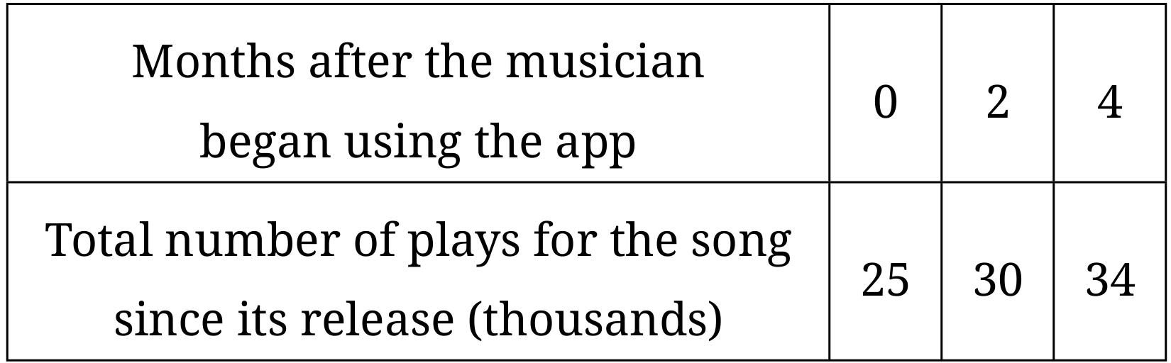
Because $ D(0) = 25 $, $ D(2) = 30 $, and $ D(4) = 34 $, the three equations are: \[ \begin{align*} a(0)^2 + b(0) + c &= 25 \\ a(2)^2 + b(2) + c &= 30 \\ a(4)^2 + b(4) + c &= 34 \end{align*} \] These simplify to: \[ \begin{align*} c &= 25 \quad \text{(1)} \\ 4a + 2b + c &= 30 \quad \text{(2)} \\ 16a + 4b + c &= 34 \quad \text{(3)} \end{align*} \] ✅ Answer: $\boxed{c=25, \; 4a+2b+c=30, \; 16a+4b+c=34}$

(ii)
Substitute $ c = 25 $ into (2) and (3): \[ \begin{align*} 4a + 2b &= 5 \quad \text{(2′)} \\ 16a + 4b &= 9 \quad \text{(3′)} \end{align*} \] Multiply (2′) by 2: $ 8a + 4b = 10 $.
Subtract this from (3′): $ (16a+4b) – (8a+4b) = 9 – 10 $ gives $ 8a = -1 $, so $ a = -\frac{1}{8} = -0.125 $.
Substitute into (2′): $ 4(-0.125) + 2b = 5 $ gives $ -0.5 + 2b = 5 $, so $ 2b = 5.5 $, $ b = 2.75 $.
✅ Answer: $\boxed{a = -0.125, \; b = 2.75, \; c = 25}$
Thus, $ D(t) = -0.125t^2 + 2.75t + 25 $.

(i)
Average rate of change from $ t=0 $ to $ t=4 $: \[ \frac{D(4)-D(0)}{4-0} = \frac{34 – 25}{4} = \frac{9}{4} = 2.25 \] ✅ Answer: $\boxed{2.25}$ thousand plays per month.

(ii)
Using the average rate of change, the linear estimate is $ A_t = D(0) + 2.25t = 25 + 2.25t $.
For $ t = 1.5 $: \[ A_{1.5} = 25 + 2.25(1.5) = 25 + 3.375 = 28.375 \] ✅ Answer: $\boxed{28.375}$ thousand plays.

(iii)
The estimate $ A_t $ is the $ y $-coordinate of a point on the secant line passing through $ (0, D(0)) $ and $ (4, D(4)) $.
Since $ D(t) $ is a quadratic with $ a = -0.125 < 0 $, its graph is concave down on $ 0 < t < 4 $.
For a concave-down function over an interval, the secant line connecting the endpoints lies below the graph of the function for all $ t $ in the open interval $ (0, 4) $.
Therefore, $ A_t < D(t) $ for all $ t $ where $ 0 < t < 4 $.
✅ Explanation: Concave-down shape places the secant line below the curve.

C.
The quadratic $ D(t) = -0.125t^2 + 2.75t + 25 $ has $ a < 0 $, so it has an absolute maximum (vertex).
Find vertex: $ t = -\frac{b}{2a} = -\frac{2.75}{2(-0.125)} = \frac{2.75}{0.25} = 11 $ months.
In the context, $ D(t) $ models the total number of plays since release, which cannot decrease. However, the quadratic model decreases after $ t = 11 $ (its maximum), which would imply the total plays go down—impossible in reality.
Therefore, the model is only valid up to the time it reaches its maximum. The domain of $ D $ should be restricted to $ t \le 11 $ months (or until the maximum is reached) to ensure the total plays are non-decreasing.
✅ Explanation: The absolute maximum at $ t = 11 $ gives a right endpoint for the domain because the total plays cannot decrease after that time.

Question

A student won $500$ in an art contest. At first, the student kept the money in a desk. After $10$ months, the student deposited the money in a savings account that earned interest. Six months after depositing the money ($t = 6$), the amount in the account is $508.67$. Twelve months after depositing the money ($t = 12$), the amount in the account is $517.50$.

The amount of money the student has can be modeled by the piecewise function $M$ given by: $$M(t) = \begin{cases} 500 & \text{for } -10 \le t < 0 \\ ab^{(t/12)} & \text{for } t \ge 0 \end{cases}$$ where $M(t)$ is the amount, in dollars, at time $t$ months since the $500$ was deposited into the savings account. A negative value for $t$ represents the number of months before the student deposited the $500$ into the savings account.

Part A

(i) Use the given data to write two equations that can be used to find the values for constants $a$ and $b$ in the expression for $M(t)$.

(ii) Find the values for $a$ and $b$ as decimal approximations.

Part B

(i) Use the given data to find the average rate of change of the amount of money the student has, in dollars per month, from $t = -2$ to $t = 12$ months. Express your answer as a decimal approximation. Show the computations that lead to your answer.

(ii) Use $M(12)$ and the average rate of change found in (i) to estimate the amount of money, in dollars, the student has when $t = 20$ months. Show the work that leads to your answer.

(iii) Let $A(t)$ be the estimate of the amount of money, in dollars, the student has at time $t$ months using the average rate of change found in (i). If $A(t)$ is used to estimate values for $M(t)$ for $t > 12$, the error in the estimates will increase as $t$ increases. Explain why this is true.

Part C

The student plans to close the account when the amount of money in the account reaches $565$. Explain how this information can be used to determine the domain limitations for the model $M$.

▶️ Answer/Explanation

Detailed solution

Part A

(i)
Using the data $M(6) = 508.67$ and $M(12) = 517.50$:
$ab^{(6/12)} = 508.67$ (or $ab^{0.5} = 508.67$)
$ab^{(12/12)} = 517.50$ (or $ab = 517.50$)

(ii)
Divide the second equation by the first: $\frac{ab}{ab^{0.5}} = \frac{517.50}{508.67}$
$b^{0.5} \approx 1.017359…$
$b \approx (1.017359…)^2 \approx 1.035019…$
Using $ab = 517.50 \implies a = \frac{517.50}{1.035019…} \approx 500$
Final values: $a \approx 500.00$ and $b \approx 1.035$

Part B

(i)
$t = -2$ falls in the interval $-10 \le t < 0$, so $M(-2) = 500$.
$t = 12$ is given as $M(12) = 517.50$.
Average Rate of Change $= \frac{M(12) – M(-2)}{12 – (-2)}$
$= \frac{517.50 – 500}{12 + 2}$
$= \frac{17.50}{14} = 1.25$ dollars per month.

(ii)
The linear estimate $A(t)$ uses the point $(12, 517.50)$ and slope $1.25$.
$A(20) = M(12) + 1.25(20 – 12)$
$A(20) = 517.50 + 1.25(8)$
$A(20) = 517.50 + 10 = 527.50$ dollars.

(iii)
The model $M(t)$ for $t \ge 0$ is an exponential function ($b > 1$), which is concave up.
The estimate $A(t)$ is a linear function (a secant line).
Since $M(t)$ is increasing at an increasing rate (exponential growth), the linear model will fall further behind the actual values as $t$ increases.

Part C

The model is only valid as long as the account is open.
Setting $M(t) = 565$ allows us to solve for the maximum value of $t$.
$500(1.035)^{(t/12)} = 565$
This value of $t$ serves as the upper bound (maximum) for the domain of the model $M$.

Question

A market analyst working for a small appliance manufacturer finds that if the firm produces and sells $x$ blenders annually, the total profit (in dollars) is $P(x) = -0.0013x^3 + 0.3507x^2 – 0.4591x – 421.888$. (4 marks each part)

a. Use a graphing device to help graph the polynomial function $P$.

b. Find the average rate of change of $P$ between two relative (local) extrema when $0 < x < 200$.

c. Find the equation of the secant line of the graph of $P$ between the two points in part b.

d. The inflection point of a function is the point on the graph where the graph changes concavity. Find out the inflection point of the graph of $P$.

e. How will the rate of change vary before and after the inflection point?

▶️ Answer/Explanation

Detailed solution

a. Graphing the function
Using a graphing utility for $P(x) = -0.0013x^3 + 0.3507x^2 – 0.4591x – 421.888$ on the interval $[0, 200]$ reveals a cubic curve shape.
The graph starts with a slight dip to a local minimum near $x=0$, then rises steeply to a local maximum near $x=180$, before falling again.

b. Average rate of change between extrema
First, find the derivative: $P'(x) = -0.0039x^2 + 0.7014x – 0.4591$.
Set $P'(x) = 0$ and use the quadratic formula to find the extrema: $x \approx 0.66$ (local min) and $x \approx 179.19$ (local max).
Calculate the profit at these points: $P(0.66) \approx -422.04$ and $P(179.19) \approx 3276.57$.
The average rate of change is: $\frac{3276.57 – (-422.04)}{179.19 – 0.66} = \frac{3698.61}{178.53} \approx 20.72$.

c. Equation of the secant line
The slope $m$ was found in part (b) to be approximately $20.72$.
Using the point-slope form $y – y_1 = m(x – x_1)$ with the minimum point $(0.66, -422.04)$:
$y – (-422.04) = 20.72(x – 0.66)$
$y = 20.72x – 13.68 – 422.04$
The equation is approximately $y = 20.72x – 435.72$.

d. Inflection point
Find the second derivative: $P”(x) = -0.0078x + 0.7014$.
Set $P”(x) = 0$ to find the change in concavity: $0 = -0.0078x + 0.7014 \Rightarrow x = \frac{0.7014}{0.0078} \approx 89.92$.
Find the corresponding y-value: $P(89.92) \approx 1427.27$.
The inflection point is approximately $(89.92, 1427.27)$.

e. Variation of rate of change
The rate of change is represented by the derivative, $P'(x)$.
Before the inflection point ($x < 89.92$), the graph is concave up ($P”(x) > 0$), so the rate of change is increasing.
After the inflection point ($x > 89.92$), the graph is concave down ($P”(x) < 0$), so the rate of change is decreasing.

Question

The Chinese bamboo tree exhibits a unique growth pattern. Once a seed has been planted, the Chinese bamboo tree does not break through the ground for several years. However, once it breaks through the ground, the Chinese bamboo tree grows exponentially. In one particular experiment, a group of biologists recorded the height of a Chinese bamboo tree once it broke through the ground. After one week ($t = 1$), the Chinese bamboo tree measured 3 feet, and after five weeks ($t = 5$), the same tree measured 89 feet.

The height of the Chinese bamboo tree can be modeled by the function $H$ given by $H(t) = ab^x$, where $H(t)$ is the height of the tree, in feet, $t$ weeks after it first breaks ground.

(A) (i) Use the given data to write two equations that can be used to find the values for constants $a$ and $b$ in the expression for $H(t)$.

(ii) Find the values for $a$ and $b$.

(B) (i) Use the given data to find the average rate of change of the height of the Chinese bamboo tree, in feet per week, from $t = 1$ to $t = 5$ weeks. Express your answer as a decimal approximation. Show the computations that lead to your answer.

(ii) Interpret the meaning of your answer from (i) in the context of the problem.

(iii) Consider the average rates of change of $H$ from $t = 5$ to $t = p$ weeks, where $p > 5$. Are these average rates of change less than or greater than the average rate of change from $t = 1$ to $t = 5$ weeks found in (i)? Explain your reasoning.

(C) For which $t$-value, $t = 4$ weeks or $t = 11$ weeks, should the biologists have more confidence in when using the model $H$? Give a reason for your answer in the context of the problem.

▶️ Answer/Explanation

Detailed solution

(A)(i) Equations
Substituting the points $(1, 3)$ and $(5, 89)$ into $H(t) = ab^t$:
1. $3 = ab^1$ (or $3 = ab$)
2. $89 = ab^5$

(A)(ii) Values for a and b
Dividing equation 2 by equation 1: $\frac{ab^5}{ab} = \frac{89}{3} \implies b^4 = 29.67$.
Solving for $b$: $b = (29.67)^{0.25} \approx 2.33$.
Solving for $a$: $a = \frac{3}{2.33} \approx 1.29$.

(B)(i) Average Rate of Change
$\text{Rate} = \frac{H(5) – H(1)}{5 – 1} = \frac{89 – 3}{4} = \frac{86}{4} = 21.5$
Answer: 21.5 feet per week.

(B)(ii) Interpretation
The answer indicates that between the first and fifth weeks, the bamboo tree grew at an average speed of 21.5 feet per week.

(B)(iii) Comparison
Greater. The function represents exponential growth ($b > 1$), which is concave up. This means the rate of growth increases over time, so the rate after week 5 will be steeper than the rate before week 5.

(C) Confidence
$t = 4$ weeks.
The biologists should be more confident in $t=4$ because it is an interpolation (within the observed data range). $t=11$ is an extrapolation; biological growth cannot remain exponential indefinitely, so the model is likely inaccurate that far out.

AP Precalculus -1.3 Rates of Change in Linear and Quadratic Functions- FRQ Exam Style Questions - Effective Fall 2023