Average Rate of Change for Linear Functions
A linear function has a constant rate of change, meaning that its output changes at a steady rate as the input changes.
For a linear function written in the form \( f(x) = mx + b \), the average rate of change over any input interval is the same.
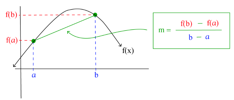
\( \text{Average rate of change} = \dfrac{f(b) – f(a)}{b – a} = m \)
This constant value \( m \) is the slope of the line and does not depend on the choice of the interval.
Graphically, this means that the graph of a linear function is a straight line with the same steepness everywhere.
Example:
Find the average rate of change of \( f(x) = 4x – 1 \) over the intervals \( [1, 3] \) and \( [3, 6] \).
▶️ Answer/Explanation
Interval \( [1, 3] \)
\( f(3) = 11 \), \( f(1) = 3 \)
\( \dfrac{11 – 3}{3 – 1} = \dfrac{8}{2} = 4 \)
Interval \( [3, 6] \)
\( f(6) = 23 \), \( f(3) = 11 \)
\( \dfrac{23 – 11}{6 – 3} = \dfrac{12}{3} = 4 \)
Conclusion
The average rate of change is 4 on both intervals, showing that it is constant.
Example:
A taxi charges a base fee plus a constant cost per kilometer. The cost function is \( C(x) = 50 + 10x \), where \( x \) is the distance traveled in kilometers. Explain why the average rate of change is constant.
▶️ Answer/Explanation
The coefficient of \( x \) is 10, which represents the cost per kilometer.
For any two distances \( a \) and \( b \),
\( \dfrac{C(b) – C(a)}{b – a} = 10 \)
This value does not change with the interval, so the average rate of change is constant.
Rates of Change of Average Rates for Quadratic Functions
A quadratic function is a function of the form \( f(x) = ax^2 + bx + c \), where \( a \ne 0 \).
For quadratic functions, the average rates of change over consecutive equal-length input intervals are not constant.
Instead, these average rates of change can be described by a linear function.
Because a linear function changes at a constant rate, the average rates of change for a quadratic function are said to be changing at a constant rate.
For an interval of length \( h \), the average rate of change from \( x \) to \( x + h \) is given by
\( \dfrac{f(x+h) – f(x)}{h} \)
When \( f(x) \) is quadratic, this expression simplifies to a linear expression in \( x \), showing a constant rate of change in the average rates.
Example:
Let \( f(x) = x^2 \). Find the average rates of change over consecutive unit intervals and describe how they change.
▶️ Answer/Explanation
Interval \( [0,1] \)
\( \dfrac{1 – 0}{1} = 1 \)
Interval \( [1,2] \)
\( \dfrac{4 – 1}{1} = 3 \)
Interval \( [2,3] \)
\( \dfrac{9 – 4}{1} = 5 \)
Conclusion
The average rates of change are 1, 3, and 5, which increase by a constant amount of 2. Therefore, they are changing at a constant rate.
Example:
Let \( g(x) = 2x^2 – 3x \). Show that the average rate of change over consecutive unit intervals changes at a constant rate.
▶️ Answer/Explanation
Average rate of change from \( x \) to \( x+1 \)
\( \dfrac{g(x+1) – g(x)}{1} \)
Compute \( g(x+1) \):
\( 2(x+1)^2 – 3(x+1) = 2x^2 + 4x + 2 – 3x – 3 \)
Subtract \( g(x) = 2x^2 – 3x \):
\( (2x^2 + x – 1) – (2x^2 – 3x) = 4x – 1 \)
Conclusion
The average rate of change is \( 4x – 1 \), which is linear. Therefore, the average rates of change are changing at a constant rate.
Average Rate of Change and Secant Lines
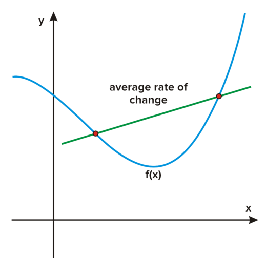
The average rate of change of a function \( f(x) \) over the closed interval \( [a, b] \) is the slope of the secant line connecting the points \( (a, f(a)) \) and \( (b, f(b)) \) on the graph of the function.
A secant line is a straight line that passes through two points on a curve.
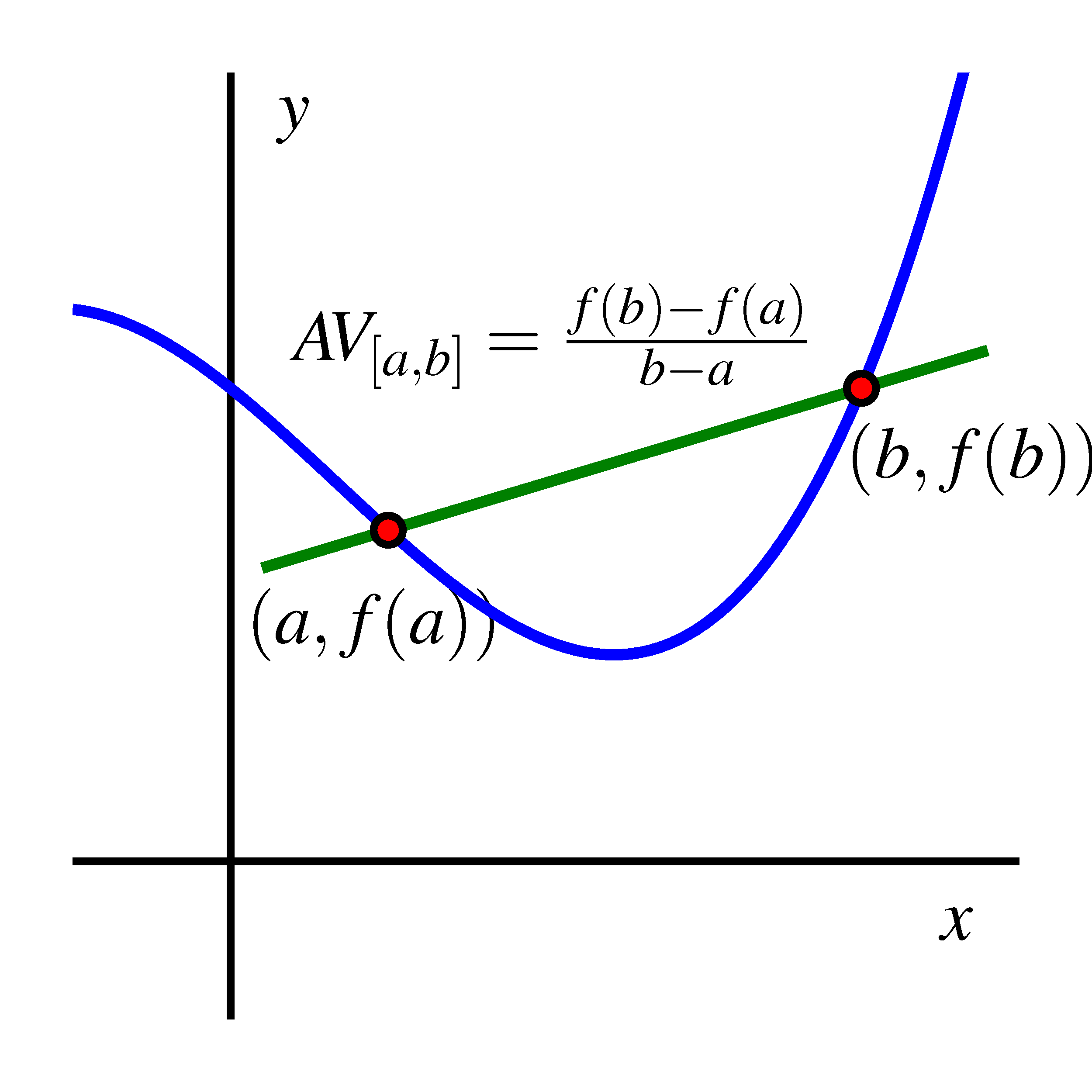
\( \text{Average rate of change on } [a, b] = \dfrac{f(b) – f(a)}{b – a} \)
This slope represents the constant rate of change that would produce the same overall change in output over the interval.
Graphically, the secant line approximates the behavior of the function over the interval.
Example:
Find the average rate of change of \( f(x) = x^2 \) over the interval \( [1, 4] \) and interpret it as a secant line.
▶️ Answer/Explanation
Compute function values
\( f(4) = 16 \)
\( f(1) = 1 \)
Compute average rate of change
\( \dfrac{16 – 1}{4 – 1} = \dfrac{15}{3} = 5 \)
Interpretation
The secant line connecting \( (1,1) \) and \( (4,16) \) has slope 5.
Example:
The position of a runner is given by \( s(t) = t^3 \). Find the average velocity between \( t = 2 \) and \( t = 5 \) and interpret it using a secant line.
▶️ Answer/Explanation
Compute function values
\( s(5) = 125 \)
\( s(2) = 8 \)
Compute average rate of change
\( \dfrac{125 – 8}{5 – 2} = \dfrac{117}{3} = 39 \)
Interpretation
The slope of the secant line between \( (2,8) \) and \( (5,125) \) is 39, representing the average velocity over the interval.
Concavity and Average Rate of Change
The concavity of a function describes how the graph bends and is directly related to how the average rate of change behaves over small, equal-length input intervals.
Consider average rates of change over intervals of equal length \( h \):
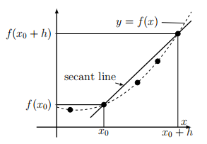
\( \text{Average rate of change from } x \text{ to } x+h = \dfrac{f(x+h) – f(x)}{h} \)
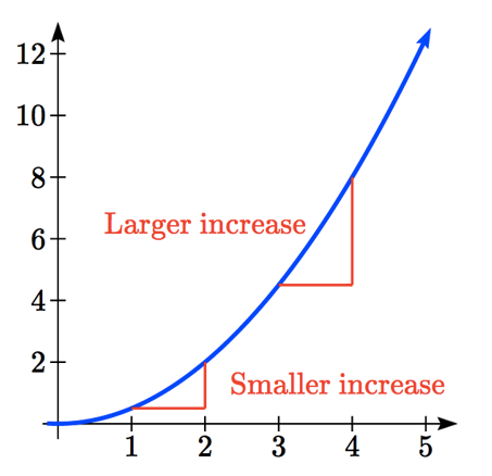
Concave Up
When the average rates of change over equal-length input intervals are increasing for all sufficiently small intervals, the graph of the function is concave up.
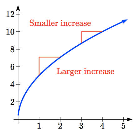
This means the slopes of secant lines are getting larger as the input increases.
Concave Down
When the average rates of change over equal-length input intervals are decreasing for all sufficiently small intervals, the graph of the function is concave down.
This means the slopes of secant lines are getting smaller as the input increases.
Example:
Explain why the function \( f(x) = x^2 \) is concave up.
▶️ Answer/Explanation
Consider consecutive unit intervals.
Average rate of change on \( [0,1] \): \( 1 \)
Average rate of change on \( [1,2] \): \( 3 \)
Average rate of change on \( [2,3] \): \( 5 \)
Since the average rates of change are increasing, the graph bends upward.
Therefore, the graph of \( f(x) = x^2 \) is concave up.
Example:
Explain why the function \( g(x) = -x^2 + 4 \) is concave down.
▶️ Answer/Explanation
Consider consecutive unit intervals.
Average rate of change on \( [0,1] \): \( -1 \)
Average rate of change on \( [1,2] \): \( -3 \)
Average rate of change on \( [2,3] \): \( -5 \)
Since the average rates of change are decreasing, the graph bends downward.
Therefore, the graph of \( g(x) = -x^2 + 4 \) is concave down.