Zeros, Roots, and Linear Factors of Polynomial Functions
Let \( p(x) \) be a polynomial function.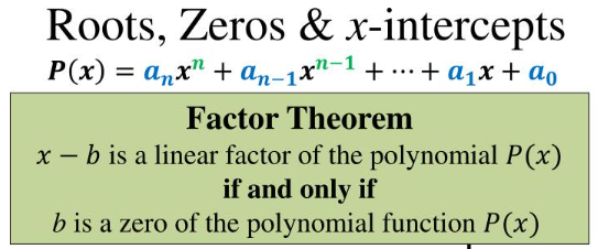
If \( a \) is a complex number such that
\( p(a) = 0 \)
then \( a \) is called a zero of the polynomial function \( p \), or equivalently, a root of the equation \( p(x) = 0 \).
Zeros and Linear Factors
If \( a \) is a real number, then
\( (x – a) \) is a linear factor of \( p(x) \) if and only if \( a \) is a zero of \( p(x) \).
This means:
If \( p(a) = 0 \), then \( (x – a) \) divides \( p(x) \).
If \( (x – a) \) is a factor of \( p(x) \), then \( p(a) = 0 \).
This relationship is known as the Factor Theorem.
Example:
Let \( p(x) = x^2 – 5x + 6 \).
Find the zeros of the polynomial and identify the corresponding linear factors.
▶️ Answer/Explanation
Factor the polynomial.
\( x^2 – 5x + 6 = (x – 2)(x – 3) \)
Set each factor equal to zero.
\( x – 2 = 0 \Rightarrow x = 2 \)
\( x – 3 = 0 \Rightarrow x = 3 \)
Conclusion
The zeros are \( x = 2 \) and \( x = 3 \), and the corresponding linear factors are \( (x – 2) \) and \( (x – 3) \).
Example:
Suppose \( (x + 1) \) is a factor of the polynomial \( p(x) = x^3 + ax^2 – 5x – 5 \).
Find the value of \( a \).
▶️ Answer/Explanation
If \( (x + 1) \) is a factor, then \( x = -1 \) is a zero.
So \( p(-1) = 0 \).
Substitute \( x = -1 \):
\( (-1)^3 + a(-1)^2 – 5(-1) – 5 = -1 + a + 5 – 5 \)
\( = a – 1 \)
Set equal to zero:
\( a – 1 = 0 \Rightarrow a = 1 \)
Conclusion
The value of \( a \) is 1.
Multiplicity of Zeros of Polynomial Functions
Let \( p(x) \) be a polynomial function.
If a linear factor \( (x – a) \) appears repeatedly in the factorization of \( p(x) \), then the corresponding zero \( a \) has a multiplicity equal to the number of times the factor appears.
If \( (x – a)^n \) is a factor of \( p(x) \), then \( a \) is a zero of multiplicity \( n \).
Multiplicity describes how the graph behaves near the zero:
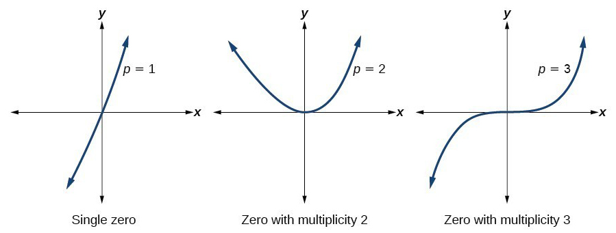
Odd multiplicity: the graph crosses the x-axis
Even multiplicity: the graph touches the x-axis and turns around
Total Number of Zeros
A polynomial function of degree \( n \) has exactly \( n \) complex zeros, when counting multiplicities.
These zeros may be real or complex, and repeated zeros are counted according to their multiplicities.
Example:
Consider the polynomial \( p(x) = (x – 2)^3(x + 1) \).
Identify the zeros and their multiplicities.
▶️ Answer/Explanation
Set each factor equal to zero.
\( x – 2 = 0 \Rightarrow x = 2 \)
The factor \( (x – 2)^3 \) appears three times, so \( x = 2 \) has multiplicity 3.
\( x + 1 = 0 \Rightarrow x = -1 \)
The factor \( (x + 1) \) appears once, so \( x = -1 \) has multiplicity 1.
Conclusion
The polynomial has degree 4 and exactly 4 zeros when counting multiplicities.
Example:
A polynomial of degree 5 has zeros at \( x = 1 \) with multiplicity 2 and \( x = -3 \) with multiplicity 1.
How many additional zeros must the polynomial have?
▶️ Answer/Explanation
The total number of zeros, counting multiplicities, must equal the degree.
Current multiplicities:
\( 2 + 1 = 3 \)
Since the degree is 5, there must be
\( 5 – 3 = 2 \)
additional zeros, which may be real or complex.
Conclusion
The polynomial must have two more zeros to account for all five zeros.
Real Zeros, X-Intercepts, and Polynomial Inequalities
Let \( p(x) \) be a polynomial function.
If \( a \) is a real zero of \( p(x) \), then
\( p(a) = 0 \)
This means the graph of \( y = p(x) \) intersects the x-axis at the point \( (a, 0) \).
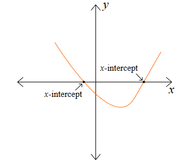
Therefore, every real zero of a polynomial corresponds to an x-intercept of its graph.
Polynomial Inequalities
Real zeros divide the real number line into intervals.
On each interval, the polynomial function is either entirely positive or entirely negative.
As a result, real zeros serve as endpoints for intervals that satisfy polynomial inequalities such as:
\( p(x) > 0 \)
\( p(x) \ge 0 \)
\( p(x) < 0 \)
\( p(x) \le 0 \)
Determining where the graph is above or below the x-axis allows us to solve these inequalities.
Example:
Consider the polynomial \( p(x) = (x – 1)(x + 2) \).
Identify the x-intercepts and the intervals where \( p(x) > 0 \).
▶️ Answer/Explanation
Set each factor equal to zero.
\( x – 1 = 0 \Rightarrow x = 1 \)
\( x + 2 = 0 \Rightarrow x = -2 \)
The x-intercepts are \( (-2, 0) \) and \( (1, 0) \).
Test intervals:
For \( x < -2 \), \( p(x) > 0 \)
For \( -2 < x < 1 \), \( p(x) < 0 \)
For \( x > 1 \), \( p(x) > 0 \)
Conclusion
The inequality \( p(x) > 0 \) is satisfied on \( (-\infty, -2) \cup (1, \infty) \).
Example:
Solve the inequality \( x^2 – 9 \le 0 \).
▶️ Answer/Explanation
Factor the expression.
\( x^2 – 9 = (x – 3)(x + 3) \)
The real zeros are \( x = -3 \) and \( x = 3 \).
Between these values, the graph is below or on the x-axis.
Conclusion
The solution is \( -3 \le x \le 3 \).
Even Multiplicity Zeros and Graph Behavior
Let \( p(x) \) be a polynomial function and let \( a \) be a real zero of \( p(x) \).
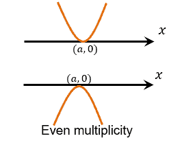
If the zero \( a \) has an even multiplicity, then the sign of the output values of the polynomial remains the same for input values near \( x = a \).
This means that the function does not cross the x-axis at \( x = a \).
Instead, the graph of the polynomial is tangent to the x-axis at \( x = a \).
Mathematically, if \( (x – a)^n \) is a factor of \( p(x) \) and \( n \) is even, then near \( x = a \), the polynomial behaves like a positive power of a squared quantity.
As a result, the graph touches the x-axis at \( x = a \) and turns around.
Example:
Consider the polynomial \( f(x) = (x – 2)^2(x + 1) \).
Describe the behavior of the graph near \( x = 2 \).
▶️ Answer/Explanation
The factor \( (x – 2)^2 \) shows that \( x = 2 \) is a zero of multiplicity 2.
Since the multiplicity is even, the sign of the function does not change near \( x = 2 \).
Therefore, the graph touches the x-axis at \( x = 2 \) and turns around instead of crossing it.
Conclusion
The graph is tangent to the x-axis at \( x = 2 \).
Example:
The polynomial \( g(x) = -3(x + 4)^4 \) has a zero at \( x = -4 \).
Explain how the graph behaves near this zero.
▶️ Answer/Explanation
The factor \( (x + 4)^4 \) shows that the zero has multiplicity 4, which is even.
Because the multiplicity is even, the sign of the function is the same on both sides of \( x = -4 \).
The graph touches the x-axis at \( x = -4 \) and turns around.
The negative leading coefficient affects the vertical direction but does not change the tangency behavior.
Conclusion
The graph is tangent to the x-axis at \( x = -4 \) and does not cross it.
Determining the Degree of a Polynomial Using Successive Differences
The degree of a polynomial function can be determined by examining how the output values change over equal-interval input values.
This method is especially useful when a polynomial is given in a table or through numerical data rather than an explicit formula.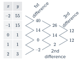
To apply this method:
1. Choose equally spaced input values.
2. Compute the first differences of the output values.
3. Continue computing successive differences.
The degree of the polynomial is the smallest value \( n \) for which the nth differences are constant.
This works because:
Constant first differences indicate a linear function.
Constant second differences indicate a quadratic function.
Constant third differences indicate a cubic function.
Example:
The table below shows values of a function for equally spaced input values.
\( \begin{array}{c|ccccc} x & 0 & 1 & 2 & 3 & 4 \\ \hline f(x) & 1 & 4 & 9 & 16 & 25 \end{array} \)
Determine the degree of the polynomial.
▶️ Answer/Explanation
First differences
\( 3,\;5,\;7,\;9 \)
Second differences
\( 2,\;2,\;2 \)
Conclusion
The second differences are constant, so the function is a quadratic polynomial (degree 2).
Example:
A function has the following output values for equally spaced inputs:
\( \begin{array}{c|ccccc} x & 1 & 2 & 3 & 4 & 5 \\ \hline f(x) & 2 & 6 & 24 & 68 & 150 \end{array} \)
Determine the degree of the polynomial.
▶️ Answer/Explanation
First differences
\( 4,\;18,\;44,\;82 \)
Second differences
\( 14,\;26,\;38 \)
Third differences
\( 12,\;12 \)
Conclusion
The third differences are constant, so the function is a cubic polynomial (degree 3).
Even and Odd Functions
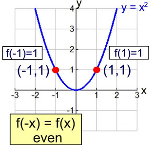
Even Functions
An even function is a function whose graph is symmetric about the y-axis, which is the line \( x = 0 \).
Analytically, a function \( f(x) \) is even if it satisfies the condition
\( f(-x) = f(x) \)
For polynomial functions, if \( n \) is even and \( a_n \ne 0 \), then a polynomial of the form
\( p(x) = a_n x^n \)
is an even function.
This occurs because raising \( -x \) to an even power gives the same result as raising \( x \) to that power.
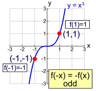
Odd Functions
An odd function is a function whose graph is symmetric about the origin, the point \( (0, 0) \).
Analytically, a function \( f(x) \) is odd if it satisfies the condition
\( f(-x) = -f(x) \)
For polynomial functions, if \( n \) is odd and \( a_n \ne 0 \), then a polynomial of the form
\( p(x) = a_n x^n \)
is an odd function.
This occurs because raising \( -x \) to an odd power produces the negative of the original value.
Example:
Determine whether the function \( f(x) = x^4 \) is even, odd, or neither.
▶️ Answer/Explanation
Evaluate \( f(-x) \).
\( f(-x) = (-x)^4 = x^4 \)
Since \( f(-x) = f(x) \), the function is even.
Conclusion
The function is an even function and is symmetric about the y-axis.
Example:
Determine whether the function \( g(x) = -3x^3 \) is even, odd, or neither.
▶️ Answer/Explanation
Evaluate \( g(-x) \).
\( g(-x) = -3(-x)^3 = 3x^3 \)
Compare with \( -g(x) \):
\( -g(x) = -(-3x^3) = 3x^3 \)
Since \( g(-x) = -g(x) \), the function is odd.
Conclusion
The function is an odd function and is symmetric about the origin.