Domain and Range of a Logarithmic Function
For a logarithmic function in general form
\( \mathrm{ \displaystyle f(x)=a\log_b x } \)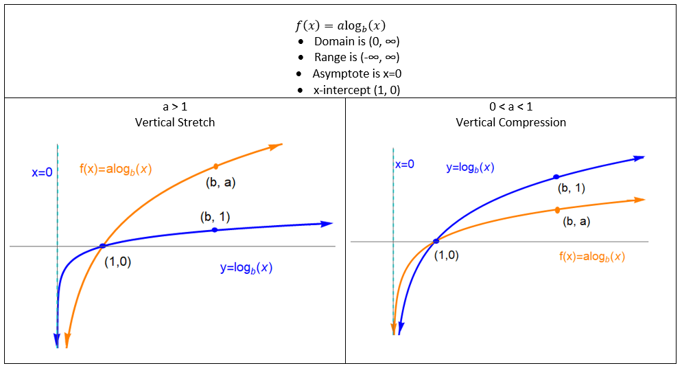
where \( \mathrm{b>0} \), \( \mathrm{b\ne1} \), and \( \mathrm{a\ne0} \):
• The domain is all real numbers greater than zero
\( \mathrm{ \displaystyle x>0 } \)
• The range is all real numbers
\( \mathrm{ \displaystyle (-\infty,\infty) } \)
The restriction \( \mathrm{x>0} \) exists because logarithms are defined only for positive inputs.
As \( \mathrm{x} \) approaches 0 from the right, the output decreases without bound, and as \( \mathrm{x} \) increases without bound, the output increases or decreases without bound depending on the base.
Example
Find the domain and range of the function
\( \mathrm{ \displaystyle f(x)=\log_5 x } \)
▶️ Answer/Explanation
Since logarithms are defined only for positive inputs,
\( \mathrm{ \displaystyle \text{Domain: } x>0 } \)
The outputs of a logarithmic function can be any real number, so
\( \mathrm{ \displaystyle \text{Range: } (-\infty,\infty) } \)
Example
Determine the domain and range of
\( \mathrm{ \displaystyle f(x)=-2\log_{10} x } \)
▶️ Answer/Explanation
The coefficient does not affect the domain, so
\( \mathrm{ \displaystyle \text{Domain: } x>0 } \)
Vertical stretching and reflection do not restrict outputs, so
\( \mathrm{ \displaystyle \text{Range: } (-\infty,\infty) } \)
Monotonicity and Concavity of Logarithmic Functions
Because logarithmic functions are the inverse functions of exponential functions, they share important global behavior properties.
For a logarithmic function in general form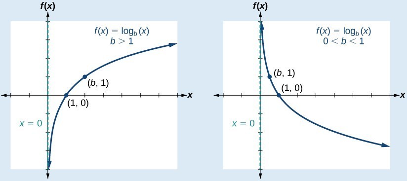
\( \mathrm{ \displaystyle f(x)=a\log_b x } \)
where \( \mathrm{b>0} \), \( \mathrm{b\ne1} \), and \( \mathrm{a\ne0} \):
• The function is always increasing if \( \mathrm{b>1} \)
• The function is always decreasing if \( \mathrm{0<b<1} \)
This means logarithmic functions are monotonic and never change direction.
Additionally, the graph of a logarithmic function is either:
• Always concave down when \( \mathrm{b>1} \)
• Always concave up when \( \mathrm{0<b<1} \)
Because the concavity does not change, logarithmic functions have no points of inflection.
Since they are always increasing or always decreasing, logarithmic functions also have no local or global extrema, except possibly when the function is restricted to a closed interval.
Example
Consider the function
\( \mathrm{ \displaystyle f(x)=\log_2 x } \)
Describe its monotonicity, concavity, and whether it has extrema or points of inflection.
▶️ Answer/Explanation
Since \( \mathrm{b=2>1} \), the function is always increasing.
The graph is concave down for all \( \mathrm{x>0} \).
Because the function never changes direction or concavity, it has:
• No extrema
• No points of inflection
Example
Consider the function
\( \mathrm{ \displaystyle f(x)=\log_{\frac12} x } \)
Explain how its graph differs from \( \mathrm{y=\log_2 x} \).
▶️ Answer/Explanation
Since \( \mathrm{0<b<1} \), the function is always decreasing.
The graph is concave up for all \( \mathrm{x>0} \).
Like all logarithmic functions, it has:
• No extrema
• No points of inflection
Additive Transformations and Logarithmic Behavior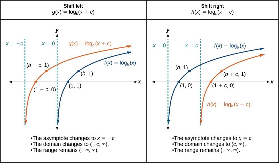
Consider a logarithmic function in general form
\( \mathrm{ \displaystyle f(x)=a\log_b x } \)
An additive transformation of this function is given by
\( \mathrm{ \displaystyle g(x)=f(x+k) } \), where \( \mathrm{k\ne0} \)
This transformation produces a horizontal translation of the graph.
For such an additive transformation of a logarithmic function:
• The input values are not proportional over equal-length output-value intervals
• The input values are not equally spaced over equal-length output-value intervals
This loss of proportionality occurs because shifting the input changes the multiplicative structure that defines logarithmic growth.
Conversely, if for an additive transformation
\( \mathrm{ \displaystyle g(x)=f(x+k) } \)
the input values are proportional over equal-length output-value intervals, then the original function \( \mathrm{f} \) must be logarithmic.
This property helps distinguish logarithmic functions from other types of functions using patterns of change.
Example
Let
\( \mathrm{ \displaystyle f(x)=\log_{10} x } \)
and consider the additive transformation
\( \mathrm{ \displaystyle g(x)=\log_{10}(x+2) } \)
Explain how the input values change over equal increases in output.
▶️ Answer/Explanation
For \( \mathrm{f(x)=\log_{10}x} \), equal increases in output correspond to multiplying inputs by 10.
After the horizontal shift, the inputs of \( \mathrm{g(x)=\log_{10}(x+2)} \) no longer change by a constant factor.
Conclusion
The additive transformation disrupts proportional input changes, even though the function remains logarithmic.
Example
Suppose a function \( \mathrm{g(x)=f(x+1)} \) has input values that are proportional over equal-length output-value intervals.
What can be concluded about the original function \( \mathrm{f} \)?
▶️ Answer/Explanation
Proportional input changes over equal output intervals are a defining characteristic of logarithmic functions.
Conclusion
If the additive transformation has this property, then the original function \( \mathrm{f} \) must be logarithmic.
Asymptotes and End Behavior of Logarithmic Functions
Logarithmic functions in general form have a limited domain and exhibit unbounded end behavior.
For a logarithmic function
\( \mathrm{ \displaystyle f(x)=a\log_b x } \)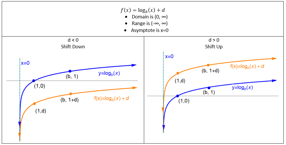
where \( \mathrm{b>0} \), \( \mathrm{b\ne1} \), and \( \mathrm{a\ne0} \):
• The domain is \( \mathrm{x>0} \)
• The graph has a vertical asymptote at
\( \mathrm{ \displaystyle x=0 } \)
As the input values approach this asymptote or increase without bound, the output values become unbounded.
End Behavior
\( \mathrm{ \displaystyle \lim_{x\to 0^+} a\log_b x=\pm\infty } \)
\( \mathrm{ \displaystyle \lim_{x\to \infty} a\log_b x=\pm\infty } \)
The sign of infinity depends on the base \( \mathrm{b} \) and the coefficient \( \mathrm{a} \):
• If \( \mathrm{b>1} \), the function increases without bound as \( \mathrm{x\to\infty} \)
• If \( \mathrm{0<b<1} \), the function decreases without bound as \( \mathrm{x\to\infty} \)
• A negative value of \( \mathrm{a} \) reflects the behavior across the x-axis
Example
Describe the asymptote and end behavior of
\( \mathrm{ \displaystyle f(x)=\log_2 x } \)
▶️ Answer/Explanation
The domain is \( \mathrm{x>0} \), so the vertical asymptote is
\( \mathrm{ \displaystyle x=0 } \)
As \( \mathrm{x\to0^+} \), the output decreases without bound:
\( \mathrm{ \displaystyle \lim_{x\to0^+}\log_2 x=-\infty } \)
As \( \mathrm{x\to\infty} \), the output increases without bound:
\( \mathrm{ \displaystyle \lim_{x\to\infty}\log_2 x=\infty } \)
Example
Determine the end behavior of
\( \mathrm{ \displaystyle f(x)=-3\log_{1/4} x } \)
▶️ Answer/Explanation
Since \( \mathrm{0<b<1} \), the logarithmic function is decreasing, and the negative coefficient reflects it.
The vertical asymptote is still
\( \mathrm{ \displaystyle x=0 } \)
Both limits are unbounded:
\( \mathrm{ \displaystyle \lim_{x\to0^+} -3\log_{1/4} x=\infty } \)
\( \mathrm{ \displaystyle \lim_{x\to\infty} -3\log_{1/4} x=-\infty } \)